Airy wave theory
This theory was first published, in correct form, by George Biddell Airy in the 19th century.
[2][3] Further, several second-order nonlinear properties of surface gravity waves, and their propagation, can be estimated from its results.
[2] Earlier attempts to describe surface gravity waves using potential flow were made by, among others, Laplace, Poisson, Cauchy and Kelland.
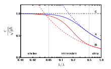
The free surface elevation η(x,t) of one wave component is sinusoidal, as a function of horizontal position x and time t: where The waves propagate along the water surface with the phase speed cp: The angular wavenumber k and frequency ω are not independent parameters (and thus also wavelength λ and period T are not independent), but are coupled.
While the surface elevation shows a propagating wave, the fluid particles are in an orbital motion.
Within the framework of Airy wave theory, the orbits are closed curves: circles in deep water and ellipses in finite depth—with the circles dying out before reaching the bottom of the fluid layer, and the ellipses becoming flatter near the bottom of the fluid layer.
In deep water, the orbit's diameter is reduced to 4% of its free-surface value at a depth of half a wavelength.
The bed being impermeable, leads to the kinematic bed boundary-condition: In case of deep water – by which is meant infinite water depth, from a mathematical point of view – the flow velocities have to go to zero in the limit as the vertical coordinate goes to minus infinity: z → −∞.
This leads to the kinematic free-surface boundary-condition: If the free surface elevation η(x,t) was a known function, this would be enough to solve the flow problem.
For a propagating wave of a single frequency – a monochromatic wave – the surface elevation is of the form:[7] The associated velocity potential, satisfying the Laplace equation (1) in the fluid interior, as well as the kinematic boundary conditions at the free surface (2), and bed (3), is: with sinh and cosh the hyperbolic sine and hyperbolic cosine function, respectively.
So angular frequency ω and wavenumber k – or equivalently period T and wavelength λ – cannot be chosen independently, but are related.
Secondly, allowance is made for a mean flow velocity U, in the horizontal direction and uniform over (independent of) depth z.
The table only gives the oscillatory parts of flow quantities – velocities, particle excursions and pressure – and not their mean value or drift.
Surface tension only has influence for short waves, with wavelengths less than a few decimeters in case of a water–air interface.
For very short wavelengths – 2 mm or less, in case of the interface between air and water – gravity effects are negligible.
For two homogeneous layers of fluids, of mean thickness h below the interface and h′ above – under the action of gravity and bounded above and below by horizontal rigid walls – the dispersion relationship ω2 = Ω2(k) for gravity waves is provided by:[16] where again ρ and ρ′ are the densities below and above the interface, while coth is the hyperbolic cotangent function.
In the table below, several second-order wave properties – as well as the dynamical equations they satisfy in case of slowly varying conditions in space and time – are given.
Further on in this section, more detailed descriptions and results are given for the general case of propagation in two-dimensional horizontal space.
The last four equations describe the evolution of slowly varying wave trains over bathymetry in interaction with the mean flow, and can be derived from a variational principle: Whitham's averaged Lagrangian method.
[19] In the mean horizontal-momentum equation, d(x) is the still water depth, that is, the bed underneath the fluid layer is located at z = −d.
[20] As can be seen above, many wave quantities like surface elevation and orbital velocity are oscillatory in nature with zero mean (within the framework of linear theory).
It is the sum of the kinetic and potential energy density, integrated over the depth of the fluid layer and averaged over the wave phase.
Using the dispersion relation, the result for surface gravity waves is: As can be seen, the mean kinetic and potential energy densities are equal.
This is a general property of energy densities of progressive linear waves in a conservative system.
[22][23] Adding potential and kinetic contributions, Epot and Ekin, the mean energy density per unit horizontal area E of the wave motion is: In case of surface tension effects not being negligible, their contribution also adds to the potential and kinetic energy densities, giving[22] so with γ the surface tension.
The equation for mass conservation is:[19][34] where h(x,t) is the mean water depth, slowly varying in space and time.


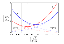
Blue lines (A): phase velocity c p , Red lines (B): group velocity c g .
Drawn lines: gravity–capillary waves.
Dashed lines: gravity waves.
Dash-dot lines: pure capillary waves.
Note: σ is surface tension in this graph.
