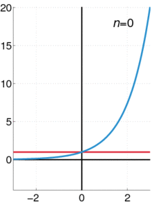
Exponential function
It is called exponential because its argument can be seen as an exponent to which a constant number e ≈ 2.718, the base, is raised.
The exponential function can be generalized to accept complex numbers as arguments.
The exponential function can be even further generalized to accept other types of arguments, such as matrices and elements of Lie algebras.
This is a second existence proof, and shows, as a byproduct, that the exponential function is defined for every
, that is, if it is obtained from exponentiation by fixing the base and letting the exponent vary.
Examples are unlimited population growth leading to Malthusian catastrophe, continuously compounded interest, and radioactive decay.
The basic properties of the exponential function (derivative and functional equation) implies immediately the third and ths last condititon Suppose that the third condition is verified, and let
The earliest occurrence of the exponential function was in Jacob Bernoulli's study of compound interests in 1683.
The exponential function is involved as follows in the computation of continuously compounded interests.
Letting the number of time intervals per year grow without bound leads to the limit definition of the exponential function,
Indeed, the exponential function is a solution of the simplest possible differential equation, namely
is an arbitrary constant and the integral denotes any antiderivative of its argument.
More generally, the solutions of every linear differential equation with constant coefficients can be expressed in terms of exponential functions and, when they are not homogeneous, antiderivatives.
This holds true also for systems of linear differential equations with constant coefficients.
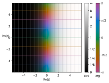
The complex exponential function can be defined in several equivalent ways that are the same as in the real case.
Complex exponential and trigonometric functions are strongly related by Euler's formula:
This formula provides the decomposition of complex exponential in real and imaginary parts:
These formulas may be used for defining trigonometric functions of a complex variable.
the graph of the exponential function is a two-dimensional surface curving through four dimensions.
domain, the following are depictions of the graph as variously projected into two or three dimensions.
axis of the graph of the real exponential function, producing a horn or funnel shape.
The fourth image shows the graph extended along the imaginary
values have been extended to ±2π, this image also better depicts the 2π periodicity in the imaginary
The power series definition of the exponential function makes sense for square matrices (for which the function is called the matrix exponential) and more generally in any unital Banach algebra B.
If xy = yx, then ex + y = exey, but this identity can fail for noncommuting x and y.
can fail for Lie algebra elements x and y that do not commute; the Baker–Campbell–Hausdorff formula supplies the necessary correction terms.
If a1, ..., an are distinct complex numbers, then ea1z, ..., eanz are linearly independent over
The Taylor series definition above is generally efficient for computing (an approximation of)
This was first implemented in 1979 in the Hewlett-Packard HP-41C calculator, and provided by several calculators,[12][13] operating systems (for example Berkeley UNIX 4.3BSD[14]), computer algebra systems, and programming languages (for example C99).
The following generalized continued fraction for ez converges more quickly:[16]