Cost curve
But in the long run, with the quantities of both labor and physical capital able to be chosen, the total cost of producing a particular output level is the result of an optimization problem: The sum of expenditures on labor (the wage rate times the chosen level of labor usage) and expenditures on capital (the unit cost of capital times the chosen level of physical capital usage) is minimized with respect to labor usage and capital usage, subject to the production function equality relating output to both input usages; then the (minimal) level of total cost is the total cost of producing the given quantity of output.
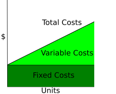
Since short-run fixed cost (FC/SRFC) does not vary with the level of output, its curve is horizontal as shown here.
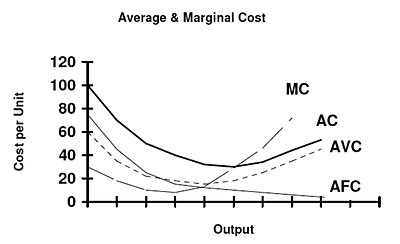
The SRAVC curve plots the short-run average variable cost against the level of output and is typically drawn as U-shaped.
However, whilst this is convenient for economic theory, it has been argued that it bears little relationship to the real world.
Some estimates show that, at least for manufacturing, the proportion of firms reporting a U-shaped cost curve is in the range of 5 to 11 percent.
From this we obtain short-run average cost, denoted either SATC or SRAC, as STC / Q: where
A short-run marginal cost (SRMC) curve graphically represents the relation between marginal (i.e., incremental) cost incurred by a firm in the short-run production of a good or service and the quantity of output produced.
This curve is constructed to capture the relation between marginal cost and the level of output, holding other variables, like technology and resource prices, constant.
Thus marginal cost initially falls, reaches a minimum value and then increases.
The long-run marginal cost curve tends to be flatter than its short-run counterpart due to increased input flexibility.
Long-run marginal cost equals short run marginal-cost at the least-long-run-average-cost level of production.
In this case, with perfect competition in the output market the long-run market equilibrium will involve all firms operating at the minimum point of their long-run average cost curves (i.e., at the borderline between economies and diseconomies of scale).
For the short run curve the initial downward slope is largely due to declining average fixed costs.
[4]: 227 With the long run curve the shape by definition reflects economies and diseconomies of scale.
[15]: 186 At low levels of production long run production functions generally exhibit increasing returns to scale, which, for firms that are perfect competitors in input markets, means that the long run average cost is falling;[4]: 227 the upward slope of the long run average cost function at higher levels of output is due to decreasing returns to scale at those output levels.
[1] Alan Blinder, former vice president of the American Economics Association, conducted the same type of survey in 1998, which involved 200 US firms in a sample that should be representative of the US economy at large.