Cumulative frequency analysis
Cumulative frequency analysis is performed to obtain insight into how often a certain phenomenon (feature) is below a certain value.
This may help in describing or explaining a situation in which the phenomenon is involved, or in planning interventions, for example in flood protection.
It can be adapted to bring in things like climate change causing wetter winters and drier summers.
Another way is to take into account the possibility that in rare cases X may assume values larger than the observed maximum Xmax.
This can be done dividing the cumulative frequency M by N+1 instead of N. The estimate then becomes: There exist also other proposals for the denominator (see plotting positions).
Probability distributions can be fitted by several methods,[2] for example: Application of both types of methods using for example often shows that a number of distributions fit the data well and do not yield significantly different results, while the differences between them may be small compared to the width of the confidence interval.
The figure gives an example of a useful introduction of such a discontinuous distribution for rainfall data in northern Peru, where the climate is subject to the behavior Pacific Ocean current El Niño.
According to the normal theory, the binomial distribution can be approximated and for large N standard deviation Sd can be calculated as follows: where Pc is the cumulative probability and N is the number of data.
It is seen that the standard deviation Sd reduces at an increasing number of observations N. The determination of the confidence interval of Pc makes use of Student's t-test (t).
Then, the lower (L) and upper (U) confidence limits of Pc in a symmetrical distribution are found from: This is known as Wald interval.
The probability of exceedance Pe (also called survival function) is found from: The return period T defined as: and indicates the expected number of observations that have to be done again to find the value of the variable in study greater than the value used for T. The upper (TU) and lower (TL) confidence limits of return periods can be found respectively as: For extreme values of the variable in study, U is close to 1 and small changes in U originate large changes in TU.
The strict notion of return period actually has a meaning only when it concerns a time-dependent phenomenon, like point rainfall.
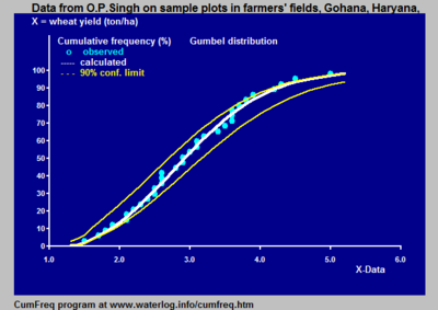
[1] The confidence belt around an experimental cumulative frequency or return period curve gives an impression of the region in which the true distribution may be found.
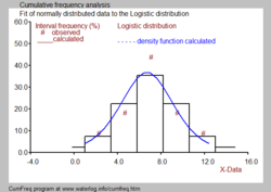
Often it is desired to combine the histogram with a probability density function as depicted in the black and white picture.