Histogram

The bins (intervals) are adjacent and are typically (but not required to be) of equal size.

If the length of the intervals on the x-axis are all 1, then a histogram is identical to a relative frequency plot.

[2][3] The term "histogram" was first introduced by Karl Pearson, the founder of mathematical statistics, in lectures delivered in 1892 at University College London.

Both of these etymologies are incorrect, and in fact Pearson, who knew Ancient Greek well, derived the term from a different if homophonous Greek root, ἱστός = "something set upright", "mast", referring to the vertical bars in the graph.

Pearson's new term was embedded in a series of other analogous neologisms, such as "stigmogram" and "radiogram".

[4] Pearson himself noted in 1895 that although the term "histogram" was new, the type of graph it designates was "a common form of graphical representation".

[5] In fact the technique of using a bar graph to represent statistical measurements was devised by the Scottish economist, William Playfair, in his Commercial and political atlas (1786).

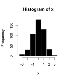
It is a good idea to plot the data using several different bin widths to learn more about it.

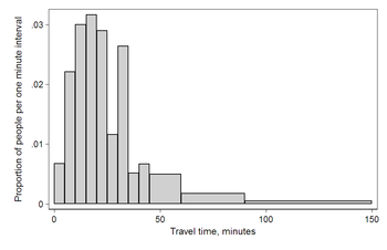
The U.S. Census Bureau found that there were 124 million people who work outside of their homes.

[6] Using their data on the time occupied by travel to work, the table below shows the absolute number of people who responded with travel times "at least 30 but less than 35 minutes" is higher than the numbers for the categories above and below it.

[citation needed] The problem of reporting values as somewhat arbitrarily rounded numbers is a common phenomenon when collecting data from people.

[citation needed] This histogram shows the number of cases per unit interval as the height of each block, so that the area of each block is equal to the number of people in the survey who fall into its category.

The area under the curve represents the total number of cases (124 million).

The intervals are placed together in order to show that the data represented by the histogram, while exclusive, is also contiguous.

)[7] The data used to construct a histogram are generated via a function mi that counts the number of observations that fall into each of the disjoint categories (known as bins).

Thus, if we let n be the total number of observations and k be the total number of bins, the histogram data mi meet the following conditions: A histogram can be thought of as a simplistic kernel density estimation, which uses a kernel to smooth frequencies over the bins.

This yields a smoother probability density function, which will in general more accurately reflect distribution of the underlying variable.

The density estimate could be plotted as an alternative to the histogram, and is usually drawn as a curve rather than a set of boxes.

Histograms are nevertheless preferred in applications, when their statistical properties need to be modeled.

The correlated variation of a kernel density estimate is very difficult to describe mathematically, while it is simple for a histogram where each bin varies independently.

Some theoreticians have attempted to determine an optimal number of bins, but these methods generally make strong assumptions about the shape of the distribution.

which takes the square root of the number of data points in the sample and rounds to the next integer.

This rule is suggested by a number of elementary statistics textbooks [12] and widely implemented in many software packages.

On the other extreme, Sturges's formula may overestimate bin width for very large datasets, resulting in oversmoothed histograms.

Scott's normal reference rule[17] is optimal for random samples of normally distributed data, in the sense that it minimizes the integrated mean squared error of the density estimate.

It replaces 3.5σ of Scott's rule with 2 IQR, which is less sensitive than the standard deviation to outliers in data.

This approach of minimizing integrated mean squared error from Scott's rule can be generalized beyond normal distributions, by using leave-one out cross validation:[21][22] Here,

independent realizations of a bounded probability distribution with smooth density.

is the "width" of the distribution (e. g., the standard deviation or the inter-quartile range), then the number of units in a bin (the frequency) is of order

This simple cubic root choice can also be applied to bins with non-constant widths.