Randomized algorithm
In some cases, probabilistic algorithms are the only practical means of solving a problem.
The number of iterations is always less than or equal to k. Taking k to be constant the run time (expected and absolute) is
In cryptographic applications, pseudo-random numbers cannot be used, since the adversary can predict them, making the algorithm effectively deterministic.
In the example above, the Las Vegas algorithm always outputs the correct answer, but its running time is a random variable.
The Monte Carlo algorithm (related to the Monte Carlo method for simulation) is guaranteed to complete in an amount of time that can be bounded by a function the input size and its parameter k, but allows a small probability of error.
Observe that any Las Vegas algorithm can be converted into a Monte Carlo algorithm (via Markov's inequality), by having it output an arbitrary, possibly incorrect answer if it fails to complete within a specified time.
Computational complexity theory models randomized algorithms as probabilistic Turing machines.
Both Las Vegas and Monte Carlo algorithms are considered, and several complexity classes are studied.
The most basic randomized complexity class is RP, which is the class of decision problems for which there is an efficient (polynomial time) randomized algorithm (or probabilistic Turing machine) which recognizes NO-instances with absolute certainty and recognizes YES-instances with a probability of at least 1/2.
The class of problems for which both YES and NO-instances are allowed to be identified with some error is called BPP.
[4] In the same year, Hoare published the quickselect algorithm,[5] which finds the median element of a list in linear expected time.
[7] In 1970, Elwyn Berlekamp introduced a randomized algorithm for efficiently computing the roots of a polynomial over a finite field.
Soon afterwards Michael O. Rabin demonstrated that the 1976 Miller's primality test could also be turned into a polynomial-time randomized algorithm.
At that time, no provably polynomial-time deterministic algorithms for primality testing were known.
One of the earliest randomized data structures is the hash table, which was introduced in 1953 by Hans Peter Luhn at IBM.
[9] Luhn's hash table used chaining to resolve collisions and was also one of the first applications of linked lists.
[9] Subsequently, in 1954, Gene Amdahl, Elaine M. McGraw, Nathaniel Rochester, and Arthur Samuel of IBM Research introduced linear probing,[9] although Andrey Ershov independently had the same idea in 1957.
Early work on randomized data structures also extended beyond hash tables.
[13] In 1989, Raimund Seidel and Cecilia R. Aragon introduced a randomized balanced search tree known as the treap.
[14] In the same year, William Pugh introduced another randomized search tree known as the skip list.
[15] Prior to the popularization of randomized algorithms in computer science, Paul Erdős popularized the use of randomized constructions as a mathematical technique for establishing the existence of mathematical objects.
[16] Erdős gave his first application of the probabilistic method in 1947, when he used a simple randomized construction to establish the existence of Ramsey graphs.
[17] He famously used a more sophisticated randomized algorithm in 1959 to establish the existence of graphs with high girth and chromatic number.
Many deterministic versions of this algorithm require O(n2) time to sort n numbers for some well-defined class of degenerate inputs (such as an already sorted array), with the specific class of inputs that generate this behavior defined by the protocol for pivot selection.
However, if the algorithm selects pivot elements uniformly at random, it has a provably high probability of finishing in O(n log n) time regardless of the characteristics of the input.
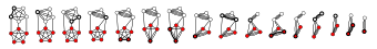
After m times executions of the outer loop, we output the minimum cut among all the results.
Consider the inner loop and let Gj denote the graph after j edge contractions, where j ∈ {0, 1, …, n − 3}.
For instance, in computational complexity, it is unknown whether P = BPP[23], i.e., we do not know whether we can take an arbitrary randomized algorithm that runs in polynomial time with a small error probability and derandomize it to run in polynomial time without using randomness.
There are specific methods that can be employed to derandomize particular randomized algorithms: When the model of computation is restricted to Turing machines, it is currently an open question whether the ability to make random choices allows some problems to be solved in polynomial time that cannot be solved in polynomial time without this ability; this is the question of whether P = BPP.
However, in other contexts, there are specific examples of problems where randomization yields strict improvements.