Equations of motion

[1] More specifically, the equations of motion describe the behavior of a physical system as a set of mathematical functions in terms of dynamic variables.

The solutions to nonlinear equations may show chaotic behavior depending on how sensitive the system is to the initial conditions.

Kinematics, dynamics and the mathematical models of the universe developed incrementally over three millennia, thanks to many thinkers, only some of whose names we know.

In antiquity, priests, astrologers and astronomers predicted solar and lunar eclipses, the solstices and the equinoxes of the Sun and the period of the Moon.

Medieval scholars in the thirteenth century — for example at the relatively new universities in Oxford and Paris — drew on ancient mathematicians (Euclid and Archimedes) and philosophers (Aristotle) to develop a new body of knowledge, now called physics.

At Oxford, Merton College sheltered a group of scholars devoted to natural science, mainly physics, astronomy and mathematics, who were of similar stature to the intellectuals at the University of Paris.

Thomas Bradwardine extended Aristotelian quantities such as distance and velocity, and assigned intensity and extension to them.

Bradwardine suggested an exponential law involving force, resistance, distance, velocity and time.

Only Domingo de Soto, a Spanish theologian, in his commentary on Aristotle's Physics published in 1545, after defining "uniform difform" motion (which is uniformly accelerated motion) – the word velocity was not used – as proportional to time, declared correctly that this kind of motion was identifiable with freely falling bodies and projectiles, without his proving these propositions or suggesting a formula relating time, velocity and distance.

Discourses such as these spread throughout Europe, shaping the work of Galileo Galilei and others, and helped in laying the foundation of kinematics.

He measured momentum by the product of velocity and weight; mass is a later concept, developed by Huygens and Newton.

In 1583, while he was praying in the cathedral at Pisa, his attention was arrested by the motion of the great lamp lighted and left swinging, referencing his own pulse for time keeping.

More careful experiments carried out by him later, and described in his Discourses, revealed the period of oscillation varies with the square root of length but is independent of the mass the pendulum.

Thus we arrive at René Descartes, Isaac Newton, Gottfried Leibniz, et al.; and the evolved forms of the equations of motion that begin to be recognized as the modern ones.

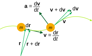
Notice that velocity always points in the direction of motion, in other words for a curved path it is the tangent vector.

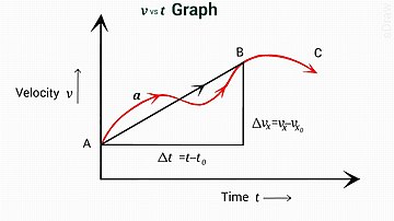
These equations apply to a particle moving linearly, in three dimensions in a straight line with constant acceleration.

In 3D space, the equations in spherical coordinates (r, θ, φ) with corresponding unit vectors êr, êθ and êφ, the position, velocity, and acceleration generalize respectively to

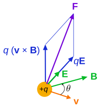
In its most general form it states the rate of change of momentum p = p(t) = mv(t) of an object equals the force F = F(x(t), v(t), t) acting on it,[13]: 1112

They also apply to each point in a mass continuum, like deformable solids or fluids, but the motion of the system must be accounted for; see material derivative.

Often there is an excess of variables to solve for the problem completely, so Newton's laws are not always the most efficient way to determine the motion of a system.

where G is the gravitational constant, M the mass of the Earth, and A = ⁠R/m⁠ is the acceleration of the projectile due to the air currents at position r and time t. The classical N-body problem for N particles each interacting with each other due to gravity is a set of N nonlinear coupled second order ODEs,

in which ⁠∂/∂q⁠ = (⁠∂/∂q1⁠, ⁠∂/∂q2⁠, …, ⁠∂/∂qN⁠) is a shorthand notation for a vector of partial derivatives with respect to the indicated variables (see for example matrix calculus for this denominator notation), and possibly time t, Setting up the Hamiltonian of the system, then substituting into the equations and evaluating the partial derivatives and simplifying, a set of coupled 2N first order ODEs in the coordinates qi and momenta pi are obtained.

Although the equation has a simple general form, for a given Hamiltonian it is actually a single first order non-linear PDE, in N + 1 variables.

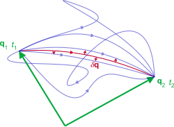
The action S allows identification of conserved quantities for mechanical systems, even when the mechanical problem itself cannot be solved fully, because any differentiable symmetry of the action of a physical system has a corresponding conservation law, a theorem due to Emmy Noether.

Combining with Newton's second law gives a first order differential equation of motion, in terms of position of the particle:

Given the mass-energy distribution provided by the stress–energy tensor T αβ, the Einstein field equations are a set of non-linear second-order partial differential equations in the metric, and imply the curvature of spacetime is equivalent to a gravitational field (see equivalence principle).

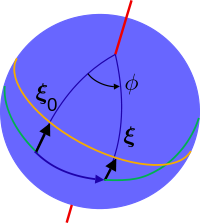
where ξα = x2α − x1α is the separation vector between two geodesics, ⁠D/ds⁠ (not just ⁠d/ds⁠) is the covariant derivative, and Rαβγδ is the Riemann curvature tensor, containing the Christoffel symbols.

[18]: 34–35 For flat spacetime, the metric is a constant tensor so the Christoffel symbols vanish, and the geodesic equation has the solutions of straight lines.

where Ψ is the wavefunction of the system, Ĥ is the quantum Hamiltonian operator, rather than a function as in classical mechanics, and ħ is the Planck constant divided by 2π.

To compare to measurements, operators for observables must be applied the quantum wavefunction according to the experiment performed, leading to either wave-like or particle-like results.