Fick's laws of diffusion
In 1855, physiologist Adolf Fick first reported[2] his now well-known laws governing the transport of mass through diffusive means.
Fick's experiments (modeled on Graham's) dealt with measuring the concentrations and fluxes of salt, diffusing between two reservoirs through tubes of water.
[3] Today, Fick's laws form the core of our understanding of diffusion in solids, liquids, and gases (in the absence of bulk fluid motion in the latter two cases).
In dilute aqueous solutions the diffusion coefficients of most ions are similar and have values that at room temperature are in the range of (0.6–2)×10−9 m2/s.
In two or more dimensions we must use ∇, the del or gradient operator, which generalises the first derivative, obtaining where J denotes the diffusion flux vector.
Another form for the first law is to write it with the primary variable as mass fraction (yi, given for example in kg/kg), then the equation changes to: where The
[8] shows in detail how the diffusion equation from the kinetic theory of gases reduces to this version of Fick's law:
is the mole fraction of species i. Fick's second law predicts how diffusion causes the concentration to change with respect to time.
Fick's second law is a special case of the convection–diffusion equation in which there is no advective flux and no net volumetric source.
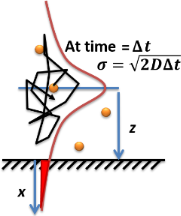
A simple case of diffusion with time t in one dimension (taken as the x-axis) from a boundary located at position x = 0, where the concentration is maintained at a value n0 is where erfc is the complementary error function.
This is the case when corrosive gases diffuse through the oxidative layer towards the metal surface (if we assume that concentration of gases in the environment is constant and the diffusion space – that is, the corrosion product layer – is semi-infinite, starting at 0 at the surface and spreading infinitely deep in the material).
For anisotropic multicomponent diffusion coefficients one needs a rank-four tensor, for example Dij,αβ, where i, j refer to the components and α, β = 1, 2, 3 correspond to the space coordinates.
Equations based on Fick's law have been commonly used to model transport processes in foods, neurons, biopolymers, pharmaceuticals, porous soils, population dynamics, nuclear materials, plasma physics, and semiconductor doping processes.
On the other hand, in some cases a "Fickian (another common approximation of the transport equation is that of the diffusion theory)" description is inadequate.
When two miscible liquids are brought into contact, and diffusion takes place, the macroscopic (or average) concentration evolves following Fick's law.
According to the fluctuation-dissipation theorem based on the Langevin equation in the long-time limit and when the particle is significantly denser than the surrounding fluid, the time-dependent diffusion constant is:[11] where (all in SI units) For a single molecule such as organic molecules or biomolecules (e.g. proteins) in water, the exponential term is negligible due to the small product of mμ in the ultrafast picosecond region, thus irrelevant to the relatively slower adsorption of diluted solute.
) in a once uniform bulk solution is solved in the above sections from Fick's equation, where C is the number concentration of adsorber molecules at
The bimolecular collision frequency related to many reactions including protein coagulation/aggregation is initially described by Smoluchowski coagulation equation proposed by Marian Smoluchowski in a seminal 1916 publication,[18] derived from Brownian motion and Fick's laws of diffusion.
In the collision theory, the traveling time between A and B is proportional to the distance which is a similar relationship for the diffusion case if the flux is fixed.
[17] Thus the concentration gradient evolution stops at the first nearest neighbor layer given a stop-time to calculate the actual flux.
He named this the critical time and derived the diffusive collision frequency in unit #/s/m3:[17] where: This equation assumes the upper limit of a diffusive collision frequency between A and B is when the first neighbor layer starts to feel the evolution of the concentration gradient, whose reaction order is 2+1/3 instead of 2.
Fick's law can be used to control and predict the diffusion by knowing how much the concentration of the dopants or chemicals move per meter and second through mathematics.
The wafer is a kind of semiconductor whose silicon substrate is coated with a layer of CVD-created polymer chain and films.
The principle of CVD relies on the gas phase and gas-solid chemical reaction to create thin films.
In CVD, reactants and products must also diffuse through a boundary layer of stagnant gas that exists next to the substrate.
In advanced semiconductor manufacturing, it is important to understand the movement at atomic scales, which is failed by continuum diffusion.
This allows us to study the effects of diffusion in a discrete manner to understand the movement of individual atoms, molecules, plasma etc.
are treated as a discrete entity, following a random walk through the CVD reactor, boundary layer, material structures etc.
Statistical analysis is done to understand variation/stochasticity arising from the random walk of the species, which in-turn affects the overall process and electrical variations.
Fick's first law can also be used to predict the changing moisture profiles across a spaghetti noodle as it hydrates during cooking.