Goodwin model (economics)

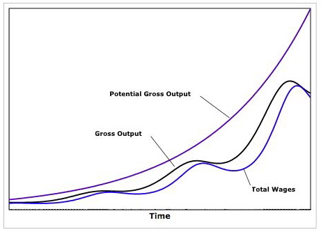
It combines aspects of the Harrod–Domar growth model with the Phillips curve to generate endogenous cycles in economic activity (output, unemployment and wages) unlike most modern macroeconomic models in which movements in economic aggregates are driven by exogenously assumed shocks.

Since Goodwin's publication in 1967, the model has been extended and applied in various ways.

for surplus) is given by The model is then defined by a set of differential equations.

Firstly, the change in labour productivity is defined by that is, steady growth, with

In other words, if the labor market is 'tight' (employment is already high) there is upward pressure on wages and vice versa in a 'lax' labor market.

Capital changes according to as the surplus is assumed to be completely invested by the capitalist.

Lastly, output changes according to that is, in proportion to the surplus invested.

The first is when and the second is when which determines the center of a family of cyclic trajectories.

Since the model cannot be solved explicitly, it is instructive to analyze the trajectory of the economy in terms of a phase diagram.

The two lines defining the center of the cycle divide the positive orthant into four regions.

The figure below indicates with arrows the movement of the economy in each region.

For example, the north-western region (high employment, low labor's share in output) the economy is moving north-east (employment is rising, worker's share is increasing).

As can be seen the Goodwin model can generate endogenous fluctuations in economic activity without relying on extraneous assumptions of outside shocks, whether on the demand or supply side.