Distributed-element filter

The filter design is usually concerned only with inductance and capacitance, but because of this mixing of elements they cannot be treated as separate "lumped" capacitors and inductors.

These discontinuities present a reactive impedance to a wavefront travelling down the line, and these reactances can be chosen by design to serve as approximations for lumped inductors, capacitors or resonators, as required by the filter.

[4] The development of distributed-element filters was spurred on by the military need for radar and electronic counter measures during World War II.

When the war ended, the technology found applications in the microwave links used by telephone companies and other organisations with large fixed-communication networks, such as television broadcasters.

Nowadays the technology can be found in several mass-produced consumer items, such as the converters (figure 1 shows an example) used with satellite television dishes.

On the other hand, antenna structure dimensions are usually comparable to λ in all frequency bands and require the distributed-element model.

[11] Mason and Sykes' work was focused on the formats of coaxial cable and balanced pairs of wires – the planar technologies were not yet in use.

[16] The difficulty with Richards' transformation from the point of view of building practical filters was that the resulting distributed-element design invariably included series connected elements.

He published a set of transformations known as Kuroda's identities in 1955, but his work was written in Japanese and it was several years before his ideas were incorporated into the English-language literature.

In 1957, Leo Young at Stanford Research Institute published a method for designing filters which started with a distributed-element prototype.

[21] This caught on rapidly, and Barrett's stripline soon had fierce commercial competition from rival planar formats, especially triplate and microstrip.

[25] Much of this work was published by the group at Stanford led by George Matthaei, and also including Leo Young mentioned above, in a landmark book which still today serves as a reference for circuit designers.

[30] More recent research has concentrated on new or variant mathematical classes of the filters, such as pseudo-elliptic, while still using the same basic topologies, or with alternative implementation technologies such as suspended stripline and finline.

[31] The initial non-military application of distributed-element filters was in the microwave links used by telecommunications companies to provide the backbone of their networks.

[33] An emerging application is in superconducting filters for use in the cellular base stations operated by mobile phone companies.

Over a narrow range of frequencies, a stub can be used as a capacitor or an inductor (its impedance is determined by its length) but over a wide band it behaves as a resonator.

Stubs can also be used in conjunction with impedance transformers to build more complex filters and, as would be expected from their resonant nature, are most useful in band-pass applications.

[40] Coupled lines (figures 3(c-e)) can also be used as filter elements; like stubs, they can act as resonators and likewise be terminated short-circuit or open-circuit.

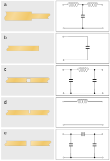
The filter consists of alternating sections of high-impedance and low-impedance lines which correspond to the series inductors and shunt capacitors in the lumped-element implementation.

In such cases, each element of the filter is λ/4 in length (where λ is the wavelength of the main-line signal to be blocked from transmission into the DC source) and the high-impedance sections of the line are made as narrow as the manufacturing technology will allow in order to maximise the inductance.

As well as the planar form shown, this structure is particularly well suited for coaxial implementations with alternating discs of metal and insulator being threaded on to the central conductor.

A stub that is narrow in comparison to λ can be taken as being connected on its centre-line and calculations based on that assumption will accurately predict filter response.

For a wide stub, however, calculations that assume the side branch is connected at a definite point on the main line leads to inaccuracies as this is no longer a good model of the transmission pattern.

It is particularly suitable for planar formats, is easily implemented with printed circuit technology and has the advantage of taking up no more space than a plain transmission line would.

The limitation of this topology is that performance (particularly insertion loss) deteriorates with increasing fractional bandwidth, and acceptable results are not obtained with a Q less than about 5.

This topology is straightforward to implement in planar technologies, but also particularly lends itself to a mechanical assembly of lines fixed inside a metal case.

As with the parallel-coupled line filter, the advantage of a mechanical arrangement that does not require insulators for support is that dielectric losses are eliminated.

The chief advantage of this design is that the upper stopband can be made very wide, that is, free of spurious passbands at all frequencies of interest.

A filter with similar properties can be constructed with λ/4 open-circuit stubs placed in series with the line and coupled together with λ/4 impedance transformers, although this structure is not possible in planar technologies.

Even structures that seem to have an "obvious" high-pass topology, such as the capacitive gap filter of figure 8, turn out to be band-pass when their behaviour for very short wavelengths is considered.

A low-noise block converter with the lid and horn removed exposing the complex circuitry inside, with the exception of the local oscillator which remains covered. The horizontal and vertical polarisation probes can be seen protruding into the circular space where the horn is normally attached. Two output connectors can be seen at the bottom of the device.
Figure 1. A circuit featuring many of the filter structures described in this article. The operating frequency of the filters is around 11 gigahertz (GHz). This circuit is described in the box below.
The PCB inside a 20GHz Agilent N9344C spectrum analyser showing various microstrip distributed-element filter technology elements
Photograph
Figure 2. A parallel-coupled lines filter in microstrip construction
A matrix of diagrams. (a1), a stripline through line with a perpendicular branch line terminated in a short-circuit strap. The length of the branch line is marked as length θ. (a2), a wire pair through line with a perpendicular branch line in parallel, terminated in a short circuit. The length of the branch line is marked as length θ. (a3), a circuit diagram of a parallel LC circuit in shunt with the line. (a4), identical to (a3). (b1), identical to (a1) but without the terminating strap. (b2), as (a2) except the branch line is terminated in an open-circuit. (b3), a circuit diagram of a series LC circuit in shunt with the line. (b4), identical to (b3). (c1), a stripline through line with a short line running parallel to it. The short line is terminated with a short-circuit strap at the left end, is left open-circuit at the right end, and is marked as length θ. (c2), a wire pair through line with a perpendicular branch line in series with the upper conductor of the through line, terminated in a short circuit. The length of the branch line is marked as length θ, as is the distance from the input to the junction with the branch line. (c3), circuit diagram of an impedance transformer in cascade with a parallel LC circuit in series with the line. (c4), identical to (b3). (d1), an input stripline is terminated in a short-circuit strap. A second line running in parallel begins at a second short-circuit strap, runs past the point where the first line terminated and then becomes the output The length of the overlap is marked as length θ. (d2), a wire pair through line with two perpendicular branch lines both terminated in short-circuits. The length of both branch lines is marked as length θ, as is the distance between the junctions of the branch lines to the through line. (d3), a circuit diagram a parallel LC circuit in shunt with the line, in cascade with an admittance transformer, in cascade with another parallel LC circuit in shunt with the line. (d4), a circuit diagram of a parallel LC circuit in shunt with the line, in cascade with a series LC circuit in series with the line. (e1), as (d1) but without the short-circuit straps. (e2), as (d2) except the branch lines terminate in open-circuits instead of short-circuits. (e3), a circuit diagram a series LC circuit in series with the line, in cascade with an impedance transformer, in cascade with another series LC circuit in series with the line. (e4), a circuit diagram of a series LC circuit in series with the line, in cascade with a parallel LC circuit in shunt with the line.
Figure 3. Some simple planar filter structures are shown in the first column. The second column shows the open-wire equivalent circuit for these structures. The third column is a semi-lumped element approximation where the elements marked K or J are impedance or admittance transformers respectively. The fourth column shows a lumped-element approximation making the further assumption that the impedance transformers are λ/4 transformers.
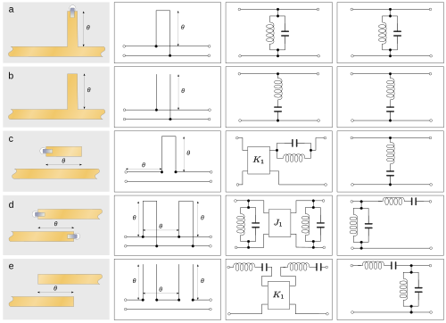
  1. A short-circuit stub in parallel with the main line.
  2. An open-circuit stub in parallel with the main line.
  3. A short-circuit line coupled to the main line.
  4. Coupled short-circuited lines.
  5. Coupled open-circuited lines.
represents a strap through the board making connection with the ground plane underneath.
A matrix of diagrams. (a1), a stripline through line that abruptly changes to a narrower width of line. (a2), a circuit diagram showing a "T" circuit consisting of a series inductor in cascade with a shunt capacitor in cascade with another series inductor. (b1), a stripline ending in an open circuit. (b2), a circuit diagram of a shunt capacitor. (c1), a stripline through line with a rectangular hole in the line. (c2), a circuit diagram showing a "Π" circuit consisting of a shunt capacitor in cascade with a series inductor in cascade with another shunt capacitor. (d1), a stripline through line with a rectangular notch cut from the upper part of the line. (d2), a circuit diagram showing an inductor in series with the line. (e1), a stripline through line with a gap cut entirely through the line. (e2), a circuit diagram of a "Π" circuit consisting of a shunt capacitor in cascade with a series capacitor in cascade with another shunt capacitor.
Figure 4. More stripline elements and their lumped-element counterparts.
  1. An abrupt stepped impedance. [ 35 ]
  2. A line coming to an abrupt end. [ 35 ]
  3. A hole or slit in a line. [ 37 ]
  4. A transverse half-slit across the line. [ 38 ]
  5. A gap in the line. [ 38 ]
A microstrip low pass filter implemented with bowtie stubs inside a 20 GHz Agilent N9344C spectrum analyser
A stripline circuit consisting of sections of line that are alternately narrower than the input line and much wider. These are all directly connected in cascade. The narrow lines are annotated as inductors and the wide lines are annotated as capacitors. An equivalent circuit is shown below the stripline diagram consisting of series inductors alternating with shunt capacitors in a ladder network.
Figure 5. Stepped-impedance low-pass filter formed from alternate high and low impedance sections of line
A stripline circuit consisting of sections of line that are narrower than the input line alternating with branch lines consisting of a narrow section of line in cascade with a wide line. An equivalent circuit is shown below the stripline diagram consisting of series inductors alternating with shunt series LC circuits in a ladder network.
Figure 6. Another form of stepped-impedance low-pass filter incorporating shunt resonators
(a), a stripline diagram consisting of a through line, which is narrower than the input and output lines, with regular perpendicular branch lines joined to alternate sides of the through line. The branch lines are wider (same width as the input and output lines) than the through line. (b), similar to (a) except that at each junction, instead of a branch line, there are two sectors of a circle joined to the through line at their apexes. (c), a gallery of stub types in stripline.
Figure 7. Low-pass filters constructed from stubs.
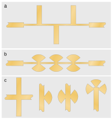
  1. Standard stubs on alternating sides of main line λ/4 apart.
  2. Similar construction using butterfly stubs.
  3. Various forms of stubs, respectively, doubled stubs in parallel, radial stub, butterfly stub (paralleled radial stubs), clover-leaf stub (triple paralleled radial stubs).
A stripline circuit consisting of a through line with regularly spaced gaps across the line
Figure 8. Capacitive gap stripline filter
A stripline circuit consisting of a number of parallel, but overlapping lines. The left end of the first line is marked as continuing (the input) and likeise the right end of the last line (the output). All other line ends are left open-circuit.
Figure 9. Stripline parallel-coupled lines filter. This filter is commonly printed at an angle as shown to minimize the board space taken up, although this is not an essential feature of the design. It is also common for the end element or the overlapping halves of the two end elements to be a narrower width for matching purposes (not shown in this diagram, see Figure 1).
A microstrip hairpin filter followed by a low pass stub filter on a PCB in a 20GHz Agilent N9344C spectrum analyser
A microstrip hairpin PCB filter implemented in an Agilent N9344C spectrum analyser
A diagram of a stripline circuit. A number of elongated "U" shapes (the hairpins) are placed in cascade, but not actually touching. The input line joins the left side of the first hairpin and the output line joins the right side of the last hairpin. The lines making up the hairpins are narrower than the main input and output lines.
Figure 10. Stripline hairpin filter
A stripline circuit consisting of a number of long parallel vertical lines. There are two horizontal lines with numerous short-circuit straps fed through holes to the board's ground plane. The vertical lines are alternately connected to the top and bottom horizontal lines. The free end of the first and last horizontal lines form the input and output respectively.
Figure 11. Stripline interdigital filter
Three Interdigital Coupled Line filters from a spectrum analyser PCB
A stripline circuit consisting of a through line with regularly spaced branch lines perpendicular to it. Each branch line (except the first and the last) extends both sides of the through line and is terminated in short-circuit straps at both ends. The first and last branch line extend to only one side, are half the length of the other branches, and have only one terminating short-circuit strap.
Figure 12. Stripline stub filter composed of λ/4 short-circuit stubs
A stripline circuit consisting of a through line with two 60° circle sectors attached to the line (one either side) by their apexes
Figure 13. Konishi's 60° butterfly stub