Lennard-Jones potential
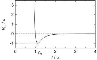
Numerous intermolecular potentials have been proposed in the past for the modeling of simple soft repulsive and attractive interactions between spherically symmetric particles, i.e. the general shape shown in the Figure.
[11] In 1924, the year that Lennard-Jones received his PhD from Cambridge University, he published[6][12] a series of landmark papers on the pair potentials that would ultimately be named for him.
[2][3][13][1] In these papers he adjusted the parameters of the potential then using the result in a model of gas viscosity, seeking a set of values consistent with experiment.
[3] In 1930, after the discovery of quantum mechanics, Fritz London showed that theory predicts the long-range attractive force should have
In 1931, Lennard-Jones applied this form of the potential to describe many properties of fluids setting the stage for many subsequent studies.
[1] Dimensionless reduced units can be defined based on the Lennard-Jones potential parameters, which is convenient for molecular simulations.
From a numerical point of view, the advantages of this unit system include computing values which are closer to unity, using simplified equations and being able to easily scale the results.
Different correction schemes have been developed to account for the influence of the long-range interactions in simulations and to sustain a sufficiently good approximation of the 'full' potential.
[14] The hypothetical true value of the observable of the Lennard-Jones potential at truly infinite cut-off distance (thermodynamic limit)
Also, the properties of the LJTS substance may furthermore be affected by the chosen simulation algorithm, i.e. MD or MC sampling (this is in general not the case for the 'full' Lennard-Jones potential).
The Lennard-Jones potential is not only of fundamental importance in computational chemistry and soft-matter physics, but also for the modeling of real substances.
It is also often used for somewhat special use cases, e.g. for studying thermophysical properties of two- or four-dimensional substances[33][34][35] (instead of the classical three spatial directions of our universe).
[13] Statistical mechanics[36] and computer simulations[15][16] can be used to study the Lennard-Jones potential and to obtain thermophysical properties of the 'Lennard-Jones substance'.
Due in part to its mathematical simplicity, the Lennard-Jones potential has been extensively used in studies on matter since the early days of computer simulation.
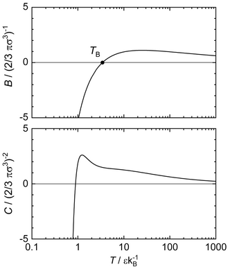
[43][21][44][45] The virial coefficients can for example be computed directly from the Lennard-potential using algebraic expressions[36] and reported data has therefore no uncertainty.
[46][32] Since the Lennard-Jonesium is the archetype for the modeling of simple yet realistic intermolecular interactions, a large number of thermophysical properties were studied and reported in the literature.
The US National Institute of Standards and Technology (NIST) provides examples of molecular dynamics and Monte Carlo codes along with results obtained from them.
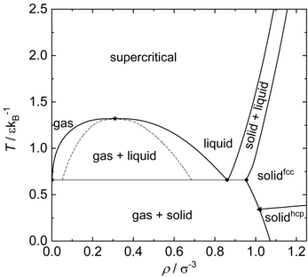
The mean intermolecular interaction of a Lennard-Jones particle strongly depends on the thermodynamic state, i.e., temperature and pressure (or density).
[21] These uncertainties can be assumed as a lower limit to the accuracy with which the critical point of fluid can be obtained from molecular simulation results.
The triple point is presently assumed to be located at The uncertainties represent the scattering of data from different authors.
The characteristic curve are required to have a negative or zero curvature throughout and a single maximum in a double-logarithmic pressure-temperature diagram.
Furthermore, Brown's characteristic curves and the virial coefficients are directly linked in the limit of the ideal gas and are therefore known exactly at
[21] Furthermore, more than 35,000 data points at homogeneous fluid states have been published over the years and recently been compiled and assessed for outliers in an open access database.
Moreover, a large number of analytical models (equations of state) have been developed for the description of the Lennard-Jones fluid (see below for details).
At low temperature and up to moderate pressure, the hcp lattice is energetically favored and therefore the equilibrium structure.
This dates back to the fundamental work of conformal solution theory of Longuet-Higgins[67] and Leland and Rowlinson and co-workers.
A large number of equations of state (EOS) for the Lennard-Jones potential/ substance have been proposed since its characterization and evaluation became available with the first computer simulations.
Three of those EOS show an unacceptable unphysical behavior in some fluid region, e.g. multiple van der Waals loops, while being elsewise reasonably precise.
There are essentially two ways the Lennard-Jones potential can be used for molecular modeling: (1) A real substance atom or molecule is modeled directly by the Lennard-Jones potential, which yields very good results for noble gases and methane, i.e. dispersively interacting spherical particles.
This is mainly due to the fact that multi-body interactions play a significant role in solid phases, which are not comprised in the Lennard-Jones potential.