Linear interpolation
In mathematics, linear interpolation is a method of curve fitting using linear polynomials to construct new data points within the range of a discrete set of known data points.
, the linear interpolant is the straight line between these points.
along the straight line is given from the equation of slopes
It is a special case of polynomial interpolation with
Outside this interval, the formula is identical to linear extrapolation.
This formula can also be understood as a weighted average.
yielding the formula for linear interpolation given above.
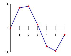
Linear interpolation on a set of data points (x0, y0), (x1, y1), ..., (xn, yn) is defined as piecewise linear, resulting from the concatenation of linear segment interpolants between each pair of data points.
This results in a continuous curve, with a discontinuous derivative (in general), thus of differentiability class
where p denotes the linear interpolation polynomial defined above:
It can be proven using Rolle's theorem that if f has a continuous second derivative, then the error is bounded by
This is intuitively correct as well: the "curvier" the function is, the worse the approximations made with simple linear interpolation become.
Linear interpolation has been used since antiquity for filling the gaps in tables.
It is believed that it was used in the Seleucid Empire (last three centuries BC) and by the Greek astronomer and mathematician Hipparchus (second century BC).
A description of linear interpolation can be found in the ancient Chinese mathematical text called The Nine Chapters on the Mathematical Art (九章算術),[1] dated from 200 BC to AD 100 and the Almagest (2nd century AD) by Ptolemy.
The basic operation of linear interpolation between two values is commonly used in computer graphics.
In that field's jargon it is sometimes called a lerp (from linear interpolation).
The term can be used as a verb or noun for the operation.
e.g. "Bresenham's algorithm lerps incrementally between the two endpoints of the line."
Lerp operations are built into the hardware of all modern computer graphics processors.
They are often used as building blocks for more complex operations: for example, a bilinear interpolation can be accomplished in three lerps.
Because this operation is cheap, it's also a good way to implement accurate lookup tables with quick lookup for smooth functions without having too many table entries.
If a C0 function is insufficient, for example if the process that has produced the data points is known to be smoother than C0, it is common to replace linear interpolation with spline interpolation or, in some cases, polynomial interpolation.
Linear interpolation as described here is for data points in one spatial dimension.
Notice, though, that these interpolants are no longer linear functions of the spatial coordinates, rather products of linear functions; this is illustrated by the clearly non-linear example of bilinear interpolation in the figure below.
Other extensions of linear interpolation can be applied to other kinds of mesh such as triangular and tetrahedral meshes, including Bézier surfaces.
These may be defined as indeed higher-dimensional piecewise linear functions (see second figure below).
Many libraries and shading languages have a "lerp" helper-function (in GLSL known instead as mix), returning an interpolation between two inputs (v0, v1) for a parameter t in the closed unit interval [0, 1].
Signatures between lerp functions are variously implemented in both the forms (v0, v1, t) and (t, v0, v1).
This lerp function is commonly used for alpha blending (the parameter "t" is the "alpha value"), and the formula may be extended to blend multiple components of a vector (such as spatial x, y, z axes or r, g, b colour components) in parallel.


Black and red / yellow / green / blue dots correspond to the interpolated point and neighbouring samples, respectively.
Their heights above the ground correspond to their values.

