Nelder–Mead method
It is a direct search method (based on function comparison) and is often applied to nonlinear optimization problems for which derivatives may not be known.
[2] The Nelder–Mead technique was proposed by John Nelder and Roger Mead in 1965,[3] as a development of the method of Spendley et al.[4] The method uses the concept of a simplex, which is a special polytope of n + 1 vertices in n dimensions.
The method approximates a local optimum of a problem with n variables when the objective function varies smoothly and is unimodal.
Typical implementations minimize functions, and we maximize
For example, a suspension bridge engineer has to choose how thick each strut, cable, and pier must be.
Simulation of such complicated structures is often extremely computationally expensive to run, possibly taking upwards of hours per execution.
The Nelder–Mead method requires, in the original variant, no more than two evaluations per iteration, except for the shrink operation described later, which is attractive compared to some other direct-search optimization methods.
However, the overall number of iterations to proposed optimum may be high.
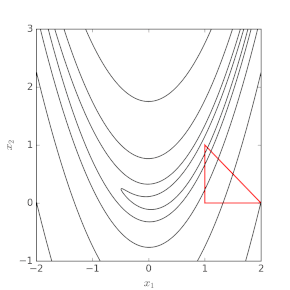
Nelder–Mead in n dimensions maintains a set of n + 1 test points arranged as a simplex.
An intuitive explanation of the algorithm from "Numerical Recipes": [5] The downhill simplex method now takes a series of steps, most steps just moving the point of the simplex where the function is largest (“highest point”) through the opposite face of the simplex to a lower point.
These steps are called reflections, and they are constructed to conserve the volume of the simplex (and hence maintain its nondegeneracy).
When it can do so, the method expands the simplex in one or another direction to take larger steps.
If there is a situation where the simplex is trying to “pass through the eye of a needle”, it contracts itself in all directions, pulling itself in around its lowest (best) point.
Unlike modern optimization methods, the Nelder–Mead heuristic can converge to a non-stationary point, unless the problem satisfies stronger conditions than are necessary for modern methods.
[2] Many variations exist depending on the actual nature of the problem being solved.
A common variant uses a constant-size, small simplex that roughly follows the gradient direction (which gives steepest descent).
Visualize a small triangle on an elevation map flip-flopping its way down a valley to a local bottom.
This, however, tends to perform poorly against the method described in this article because it makes small, unnecessary steps in areas of little interest.
is the new minimum along the vertices, we can expect to find interesting values along the direction from
, we can expect that a better value will be inside the simplex formed by all the vertices
Finally, the shrink handles the rare case that contracting away from the largest point increases
In that case we contract towards the lowest point in the expectation of finding a simpler landscape.
However, Nash notes that finite-precision arithmetic can sometimes fail to actually shrink the simplex, and implemented a check that the size is actually reduced.
Indeed, a too small initial simplex can lead to a local search, consequently the NM can get more easily stuck.
However, the original article suggested a simplex where an initial point is given as
, with the others generated with a fixed step along each dimension in turn.
Criteria are needed to break the iterative cycle.
Nelder and Mead used the sample standard deviation of the function values of the current simplex.
If these fall below some tolerance, then the cycle is stopped and the lowest point in the simplex returned as a proposed optimum.
Nash adds the test for shrinkage as another termination criterion.