Path integrals in polymer science

The modern concept of polymers as covalently bonded macromolecular structures was proposed in 1920 by Hermann Staudinger.

Because polymers are such large molecules, bordering on the macroscopic scale, their physical properties are usually too complicated for solving using deterministic methods.

Thermal fluctuations continuously affect the shape of polymers in liquid solutions, and modeling their effect requires using principles from statistical mechanics and dynamics.

The path integral approach falls in line with this basic premise and its afforded results are unvaryingly statistical averages.

Employing path integrals, problems hitherto unsolved were successfully worked out: Excluded volume, entanglement, links and knots to name a few.

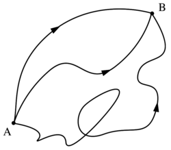
One extremely naive yet fruitful approach to quantitatively analyze the spatial structure and configuration of a polymer is the free random walk model.

In the ideal polymer model the polymer subunits are completely free to rotate with respect to each other, and therefore the process of polymerization can be looked at as a random three dimensional walk, with each monomer added corresponding to another random step of predetermined length.

The important thing to note here is that the bond position vector has a uniform distribution over a sphere of radius

acts as a parametrization variable for the polymer, describing in effect its spatial configuration, or contour.

, one can arrive at the new governing differential equation: For which the corresponding path integral is: To model a perfect rigid wall, simply set

Not only can the contour be full of bumps and twists, but their interaction with the polymer is far from the rigid mechanical idealization depicted above.

, the potential well has no bound states, meaning all eigenvalues are positive and the corresponding eigenfunction takes the asymptotic form

In our "large polymer" limit, this means that the bi-linear expansion will be dominated by the ground state, which asymptotically

takes the form: This time the configurations of the polymer are localized in a narrow layer near the surface with an effective thickness

A wide variety of adsorption problems boasting a host of "wall" geometries and interaction potentials can be solved using this method.

To obtain a quantitatively well defined result one has to use the recovered eigenfunctions and construct the corresponding configuration sum.

To better understand the problem, one can imagine a random walk chain, as previously presented, with a small hard sphere (not unlike the "specks of dust" mentioned above) at the endpoint of each monomer.

does not hold for a microscopic analysis of the polymer structure but will yield accurate results for large-scale properties.

The potential energy for such a model is given by: At thermal equilibrium one can expect the Boltzmann distribution, which indeed recovers the result above for

, the equilibrium conformational distribution described above will be modified by a Boltzmann factor: An important tool in the study of a Gaussian chain conformational distribution is the Green function, defined by the path integral quotient: The path integration is interpreted as a summation over all polymer curves

This equation has a clear physical significance, which might also serve to elucidate the concept of the path integral: The product

A particle in such an ensemble moves through space along a fluctuating orbit in a fashion that resembles a random polymer chain.

The immediate conclusion to be drawn is that large groups of polymers may also be described by a single fluctuating field.

, one usually employs a Laplace transform and considers a correlation function similar to the statistic average

[14][15] Another simplifying assumption was taken for granted in the treatment presented thus far; All models described a single polymer.

This is an important result and one immediately sees that for large chain lengths N, the overlap concentration is very small.

In the limit of very large concentrations, imagined by an almost completely filled lattice, the density fluctuations become less and less important.

The generalization for the partition function calculation is very simple and all that has to be done is to take into account the interaction between all the chain segments:

The final result corresponds to the so-called random phase approximation (RPA) which has been frequently used in solid-state physics.

To explicitly calculate the partition function using the segment density one has to switch to reciprocal space, change variables and only then execute the integration.