File dynamics
The term file dynamics is the motion of many particles in a narrow channel.
In science: in chemistry, physics, mathematics and related fields, file dynamics (sometimes called, single file dynamics) is the diffusion of N (N → ∞) identical Brownian hard spheres in a quasi-one-dimensional channel of length L (L → ∞), such that the spheres do not jump one on top of the other, and the average particle's density is approximately fixed.
The most famous statistical properties of this process is that the mean squared displacement (MSD) of a particle in the file follows,
, and its probability density function (PDF) is Gaussian in position with a variance MSD.
Indeed, file dynamics are used in modeling numerous microscopic processes:[10][11][12][13][14][15][16] the diffusion within biological and synthetic pores and porous material, the diffusion along 1D objects, such as in biological roads, the dynamics of a monomer in a polymer, etc.
, the joint probability density function (PDF) for all the particles in file, obeys a normal diffusion equation: In
Equation (1) is solved with the appropriate boundary conditions, which reflect the hard-sphere nature of the file: and with the appropriate initial condition: In a simple file, the initial density is fixed, namely,
(3), where the particles’ initial positions obey: The file diffusion coefficients are taken independently from the PDF, where Λ has a finite value that represents the fastest diffusion coefficient in the file.
In renewal-anomalous files, a random period is taken independently from a waiting time probability density function (WT-PDF; see Continuous-time Markov process for more information) of the form:
The equation of motion for the particles’ PDF in a renewal-anomalous file is obtained when convoluting the equation of motion for a Brownian file with a kernel
(8) are obtained when convoluting the boundary conditions of a Brownian file with the kernel
When each particle in the anomalous file is assigned with its own jumping time drawn form
Then, the waiting times for all the other particles are adjusted: we subtract
The most crucial difference among renewal anomalous files and anomalous files that are not renewal is that when each particle has its own clock, the particles are in fact connected also in the time domain, and the outcome is further slowness in the system (proved in the main text).
Adding all the coordinates and performing the integration in the order of faster times first (the order is determined randomly from a uniform distribution in the space of configurations) gives the full equation of motion in anomalous files of independent particles (averaging of the equation over all configurations is therefore further required).
(1)-(2) is a complete set of permutations of all initial coordinates appearing in the Gaussians,[4] Here, the index
The MSD for the tagged particle is obtained directly from Eq.
(13), the PDF of the tagged particle in the heterogeneous file follows,[5] The MSD of a tagged particle in a heterogeneous file is taken from Eq.
(8) is written in terms of the PDF that solves the un-convoluted equation, that is, the Brownian file equation; this relation is made in Laplace space: (The subscript nrml stands for normal dynamics.)
(18), one finds that the MSD of a file with normal dynamics in the power of
Solutions for such files are reached while deriving scaling laws and with numerical simulations.
Firstly, we write down the scaling law for the mean absolute displacement (MAD) in a renewal file with a constant density:[4][5][7] Here,
(20), we write a generalized scaling law for anomalous files of independent particles: The first term on the right hand side of Eq.
f(n) is the probability that accounts for the fact that for moving n anomalous independent particles in the same direction, when these particles indeed try jumping in the same direction (expressed with the term, (
), the particles in the periphery must move first so that the particles in the middle of the file will have the free space for moving, demanding faster jumping times for those in the periphery.
We calculate f(n) from the number of configurations in which the order of the particles’ jumping times enables motion; that is, an order where the faster particles are always located towards the periphery.
Yet, although not optimal, propagation is also possible in many other configurations; when m is the number of particles that move, then, where
counts the number of configurations in which those m particles around the tagged one have the optimal jumping order.
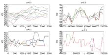
With numerical studies, one sees that anomalous files of independent particles form clusters.
The panels exhibit the phenomenon of the clustering, where the trajectories attract each other and then move pretty much together.