Routhian mechanics

In the case of Lagrangian mechanics, the generalized coordinates q1, q2, ... and the corresponding velocities dq1/dt, dq2/dt, ..., and possibly time[nb 1] t, enter the Lagrangian, where the overdots denote time derivatives.

The velocities dqi/dt are expressed as functions of their corresponding momenta by inverting their defining relation.

In this context, pi is said to be the momentum "canonically conjugate" to qi.

The Routhian is intermediate between L and H; some coordinates q1, q2, ..., qn are chosen to have corresponding generalized momenta p1, p2, ..., pn, the rest of the coordinates ζ1, ζ2, ..., ζs to have generalized velocities dζ1/dt, dζ2/dt, ..., dζs/dt, and time may appear explicitly;[1][2]

[3] Given the length of the general definition, a more compact notation is to use boldface for tuples (or vectors) of the variables, thus q = (q1, q2, ..., qn), ζ = (ζ1, ζ2, ..., ζs), p = (p1, p2, ..., pn), and d ζ/dt = (dζ1/dt, dζ2/dt, ..., dζs/dt), so that where · is the dot product defined on the tuples, for the specific example appearing here: For reference, the Euler-Lagrange equations for s degrees of freedom are a set of s coupled second order ordinary differential equations in the coordinates where j = 1, 2, ..., s, and the Hamiltonian equations for n degrees of freedom are a set of 2n coupled first order ordinary differential equations in the coordinates and momenta Below, the Routhian equations of motion are obtained in two ways, in the process other useful derivatives are found that can be used elsewhere.

Consider the case of a system with two degrees of freedom, q and ζ, with generalized velocities dq/dt and dζ/dt, and the Lagrangian is time-dependent.

(The generalization to any number of degrees of freedom follows exactly the same procedure as with two).

[4] The Lagrangian of the system will have the form The differential of L is Now change variables, from the set (q, ζ, dq/dt, dζ/dt) to (q, ζ, p, dζ/dt), simply switching the velocity dq/dt to the momentum p. This change of variables in the differentials is the Legendre transformation.

Using the definition of generalized momentum and Lagrange's equation for the coordinate q: we have and to replace pd(dq/dt) by (dq/dt)dp, recall the product rule for differentials,[nb 2] and substitute to obtain the differential of a new function in terms of the new set of variables: Introducing the Routhian where again the velocity dq/dt is a function of the momentum p, we have but from the above definition, the differential of the Routhian is Comparing the coefficients of the differentials dq, dζ, dp, d(dζ/dt), and dt, the results are Hamilton's equations for the coordinate q, and Lagrange's equation for the coordinate ζ which follow from and taking the total time derivative of the second equation and equating to the first.

Notice the Routhian replaces the Hamiltonian and Lagrangian functions in all the equations of motion.

The remaining equation states the partial time derivatives of L and R are negatives For n + s coordinates as defined above, with Routhian the equations of motion can be derived by a Legendre transformation of this Routhian as in the previous section, but another way is to simply take the partial derivatives of R with respect to the coordinates qi and ζj, momenta pi, and velocities dζj/dt, where i = 1, 2, ..., n, and j = 1, 2, ..., s. The derivatives are The first two are identically the Hamiltonian equations.

This expression requires the partial derivatives of L with respect to all the velocities dqi/dt and dζj/dt.

Under the same condition of R being time independent, the energy in terms of the Routhian is a little simpler, substituting the definition of R and the partial derivatives of R with respect to the velocities dζj/dt, Notice only the partial derivatives of R with respect to the velocities dζj/dt are needed.

The same expression for R in when s = 0 is also the Hamiltonian, so in all E = R = H. If the Routhian has explicit time dependence, the total energy of the system is not constant.

The general result is which can be derived from the total time derivative of R in the same way as for L. Often the Routhian approach may offer no advantage, but one notable case where this is useful is when a system has cyclic coordinates (also called "ignorable coordinates"), by definition those coordinates which do not appear in the original Lagrangian.

The Hamiltonian equations are useful theoretical results, but less useful in practice because coordinates and momenta are related together in the solutions - after solving the equations the coordinates and momenta must be eliminated from each other.

The Routhian approach has the best of both approaches, because cyclic coordinates can be split off to the Hamiltonian equations and eliminated, leaving behind the non cyclic coordinates to be solved from the Lagrangian equations.

Overall fewer equations need to be solved compared to the Lagrangian approach.

One general class of mechanical systems with cyclic coordinates are those with central potentials, because potentials of this form only have dependence on radial separations and no dependence on angles.

Consider a particle of mass m under the influence of a central potential V(r) in spherical polar coordinates (r, θ, φ) Notice φ is cyclic, because it does not appear in the Lagrangian.

The r equation is the θ equation is the φ equation is Consider the spherical pendulum, a mass m (known as a "pendulum bob") attached to a rigid rod of length l of negligible mass, subject to a local gravitational field g. The system rotates with angular velocity dφ/dt which is not constant.

Applying the Lagrangian approach there are two nonlinear coupled equations to solve.

Here the simple relation for local gravitational potential energy V = Mglcosθ is used where g is the acceleration due to gravity, and the centre of mass of the top is a distance l from its tip along its z′-axis.

The constant momenta are the angular momenta of the top about its axis and its precession about the vertical, respectively: From these, eliminating dψ/dt: we have and to eliminate dφ/dt, substitute this result into pψ and solve for dψ/dt to find The Routhian can be taken to be and since we have The first term is constant, and can be ignored since only the derivatives of R will enter the equations of motion.

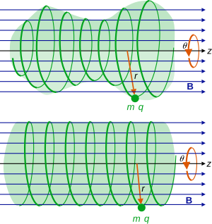
, and we can choose the axial gauge for the magnetic potential and the Lagrangian is Notice this potential has an effectively cylindrical symmetry (although it also has angular velocity dependence), since the only spatial dependence is on the radial length from an imaginary cylinder axis.

The canonical momenta conjugate to θ and z are the constants so the velocities are The angular momentum about the z axis is not pθ, but the quantity mr2dθ/dt, which is not conserved due to the contribution from the magnetic field.

It is still the case that pz is the linear or translational momentum along the z axis, which is also conserved.

The Routhian can take the form where in the last line, the pz2/2m term is a constant and can be ignored without loss of continuity.

The Hamiltonian equations for θ and z automatically vanish and do not need to be solved for.

The Lagrangian equation in r is by direct calculation which after collecting terms is and simplifying further by introducing the constants the differential equation is To see how z changes with time, integrate the momenta expression for pz above where cz is an arbitrary constant, the initial value of z to be specified in the initial conditions.