Compartmental models in epidemiology
[6] The models are most often run with ordinary differential equations (which are deterministic), but can also be used with a stochastic (random) framework, which is more realistic but much more complicated to analyze.
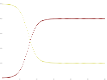
The importance of this dynamic aspect is most obvious in an endemic disease with a short infectious period, such as measles in the UK prior to the introduction of a vaccine in 1968.
(This is mathematically similar to the law of mass action in chemistry in which random collisions between molecules result in a chemical reaction and the fractional rate is proportional to the concentration of the two reactants.
This is also equivalent to the assumption that the length of time spent by an individual in the infectious state is a random variable with an exponential distribution.
This transcendental equation has a solution in terms of the Lambert W function,[17] namely This shows that at the end of an epidemic that conforms to the simple assumptions of the SIR model, unless
However, for large classes of communicable diseases it is more realistic to consider a force of infection that does not depend on the absolute number of infectious subjects, but on their fraction (with respect to the total constant population
In 2014, Harko and coauthors derived an exact so-called analytical solution (involving an integral that can only be calculated numerically) to the SIR model.
[4] These solutions may be easily understood by noting that all of the terms on the right-hand sides of the original differential equations are proportional to
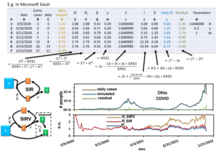
The approximant involves the Lambert W function which is part of all basic data visualization software such as Microsoft Excel, MATLAB, and Mathematica.
is usually more stable over time assuming when the infectious person shows symptoms, she/he will seek medical attention or be self-isolated.
This debate is largely on the uncertainty of the number of days reduced from after infectious or detectable whichever comes first to before a symptom shows up for an infected susceptible person.
does not tell us whether or not the spreading will speed up or slow down in the latter stages when the fraction of susceptible people in the community has dropped significantly after recovery or vaccination.
[21][22] Any point of the time can be used as the initial condition to predict the future after it using this numerical model with assumption of time-evolved parameters such as population,
[8] The model with mass-action transmission is: for which the disease-free equilibrium (DFE) is: In this case, we can derive a basic reproduction number: which has threshold properties.
In fact, independently from biologically meaningful initial values, one can show that: The point EE is called the Endemic Equilibrium (the disease is not totally eradicated and remains in the population).
Finally, it is assumed that the rate of infection and recovery is much faster than the time scale of births and deaths and therefore, these factors are ignored in this model.
We have the model: Note that denoting with N the total population it holds that: It follows that: i.e. the dynamics of infectious is ruled by a logistic function, so that
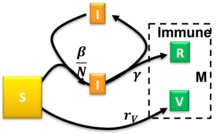
It encompasses the SIR, SIRV, SIRD, and SI models as special cases, with individual time-dependent rates governing transitions between different fractions.
[32] The case of stationary ratios allows one to construct a diagnostics method to extract analytically all SIRVD model parameters from measured COVID-19 data of a completed pandemic wave.
[32] For many infections, including measles, babies are not born into the susceptible compartment but are immune to the disease for the first few months of life due to protection from maternal antibodies (passed across the placenta and additionally through colostrum).
the condition for the global attractiveness of DFE is that the following linear system with periodic coefficients: is stable (i.e. it has its Floquet's eigenvalues inside the unit circle in the complex plane).
[33] Such Interacting Subpopulation SEIR models have been used for modeling the COVID-19 pandemic at continent scale to develop personalized, accelerated, subpopulation-targeted vaccination strategies[36] that promise a shortening of the pandemic and a reduction of case and death counts in the setting of limited access to vaccines during a wave of virus Variants of Concern.
[37] A stochastic compartment model with a transmission pathway via vectors has been developed recently in which a multiple random walkers approach is implemented to investigate the spreading dynamics in random graphs of the Watts-Strogatz and the Barabási-Albert type to mimic human mobility patterns in complex real world environments such as cities, streets, and transportation networks.
The susceptible individuals (S) can be split in three subgroups by the types of behavior: ignorant or unaware of the epidemic (Sign), rationally resistant (Sres), and exhausted (Sexh) that do not react on the external stimuli (this is a sort of refractory period).
In presence of a communicable diseases, one of the main tasks is that of eradicating it via prevention measures and, if possible, via the establishment of a mass vaccination program.
Using this strategy, the block of susceptible individuals is then immediately removed, making it possible to eliminate an infectious disease, (such as measles), from the entire population.
must hold: and the demographic equilibrium is automatically ensuring the existence of the disease-free solution: A basic reproduction number can be calculated as the spectral radius of an appropriate functional operator.
In mathematical modelling of infectious disease, the dynamics of spreading is usually described through a set of non-linear ordinary differential equations (ODE).
In stochastic models, the long-time endemic equilibrium derived above, does not hold, as there is a finite probability that the number of infected individuals drops below one in a system.
One of the possible extensions of mean-field models considers the spreading of epidemics on a network based on percolation theory concepts.