Autoregressive model
The autoregressive model specifies that the output variable depends linearly on its own previous values and on a stochastic term (an imperfectly predictable term); thus the model is in the form of a stochastic difference equation (or recurrence relation) which should not be confused with a differential equation.
Together with the moving-average (MA) model, it is a special case and key component of the more general autoregressive–moving-average (ARMA) and autoregressive integrated moving average (ARIMA) models of time series, which have a more complicated stochastic structure; it is also a special case of the vector autoregressive model (VAR), which consists of a system of more than one interlocking stochastic difference equation in more than one evolving random variable.
[1][2] This can be equivalently written using the backshift operator B as so that, moving the summation term to the left side and using polynomial notation, we have An autoregressive model can thus be viewed as the output of an all-pole infinite impulse response filter whose input is white noise.
More generally, for an AR(p) model to be weak-sense stationary, the roots of the polynomial
In an AR process, a one-time shock affects values of the evolving variable infinitely far into the future.
never ends, although if the process is stationary then the effect diminishes toward zero in the limit.
Because each shock affects X values infinitely far into the future from when they occur, any given value Xt is affected by shocks occurring infinitely far into the past.
This can also be seen by rewriting the autoregression (where the constant term has been suppressed by assuming that the variable has been measured as deviations from its mean) as When the polynomial division on the right side is carried out, the polynomial in the backshift operator applied to
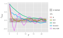
The autocorrelation function of an AR(p) process can be expressed as [citation needed] where
[citation needed] The autocorrelation function of an AR(p) process is a sum of decaying exponentials.
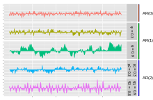
Only the error/innovation/noise term contributes to the output of the process, so in the figure, AR(0) corresponds to white noise.
approaches 1, the output gets a larger contribution from the previous term relative to the noise.
This results in a "smoothing" or integration of the output, similar to a low pass filter.
are positive, the output will resemble a low pass filter, with the high frequency part of the noise decreased.
since it is obtained as the output of a stable filter whose input is white noise.
This can be shown by noting that and then by noticing that the quantity above is a stable fixed point of this relation.
The AR(1) model is the discrete-time analogy of the continuous Ornstein-Uhlenbeck process.
It is therefore sometimes useful to understand the properties of the AR(1) model cast in an equivalent form.
There are many ways to estimate the coefficients, such as the ordinary least squares procedure or method of moments (through Yule–Walker equations).
where i = 1, ..., p. There is a direct correspondence between these parameters and the covariance function of the process, and this correspondence can be inverted to determine the parameters from the autocorrelation function (which is itself obtained from the covariances).
The full autocorrelation function can then be derived by recursively calculating [8] Examples for some Low-order AR(p) processes The above equations (the Yule–Walker equations) provide several routes to estimating the parameters of an AR(p) model, by replacing the theoretical covariances with estimated values.
Two distinct variants of maximum likelihood are available: in one (broadly equivalent to the forward prediction least squares scheme) the likelihood function considered is that corresponding to the conditional distribution of later values in the series given the initial p values in the series; in the second, the likelihood function considered is that corresponding to the unconditional joint distribution of all the values in the observed series.
Substantial differences in the results of these approaches can occur if the observed series is short, or if the process is close to non-stationarity.
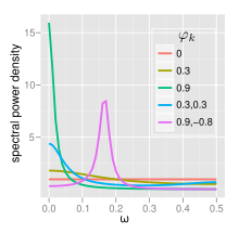
The power spectral density (PSD) of an AR(p) process with noise variance
is[8] For white noise (AR(0)) For AR(1) The behavior of an AR(2) process is determined entirely by the roots of it characteristic equation, which is expressed in terms of the lag operator as: or equivalently by the poles of its transfer function, which is defined in the Z domain by: It follows that the poles are values of z satisfying: which yields:
are the reciprocals of the characteristic roots, as well as the eigenvalues of the temporal update matrix: AR(2) processes can be split into three groups depending on the characteristics of their roots/poles: with bandwidth about the peak inversely proportional to the moduli of the poles: The terms involving square roots are all real in the case of complex poles since they exist only when
Otherwise the process has real roots, and: The process is non-stationary when the poles are on or outside the unit circle, or equivalently when the characteristic roots are on or inside the unit circle.
The full PSD function can be expressed in real form as: The impulse response of a system is the change in an evolving variable in response to a change in the value of a shock term k periods earlier, as a function of k. Since the AR model is a special case of the vector autoregressive model, the computation of the impulse response in vector autoregression#impulse response applies here.
First use t to refer to the first period for which data is not yet available; substitute the known preceding values Xt-i for i=1, ..., p into the autoregressive equation while setting the error term
Each of the last three can be quantified and combined to give a confidence interval for the n-step-ahead predictions; the confidence interval will become wider as n increases because of the use of an increasing number of estimated values for the right-side variables.