Conditional probability
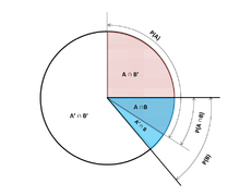
In this situation, the event A can be analyzed by a conditional probability with respect to B.
If the event of interest is A and the event B is known or assumed to have occurred, "the conditional probability of A given B", or "the probability of A under the condition B", is usually written as P(A|B)[2] or occasionally PB(A).
This can also be understood as the fraction of probability B that intersects with A, or the ratio of the probabilities of both events happening to the "given" one happening (how many times A occurs rather than not assuming B has occurred):
Alternatively, if a person is tested as positive for dengue fever, they may have only a 15% chance of actually having this rare disease due to high false positive rates.
It should be apparent now that falsely equating the two probabilities can lead to various errors of reasoning, which is commonly seen through base rate fallacies.
Therefore, it can be useful to reverse or convert a conditional probability using Bayes' theorem:
[5] A is assumed to be the set of all possible outcomes of an experiment or random trial that has a restricted or reduced sample space.
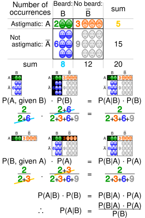
, the probability at which A and B occur together, and the probability of B:[2][6][7] For a sample space consisting of equal likelihood outcomes, the probability of the event A is understood as the fraction of the number of outcomes in A to the number of all outcomes in the sample space.
Additionally, this may be preferred philosophically; under major probability interpretations, such as the subjective theory, conditional probability is considered a primitive entity.
We can then take the limit For example, if two continuous random variables X and Y have a joint density
are identical but the resulting limits are not: The Borel–Kolmogorov paradox demonstrates this with a geometrical argument.
Let X be a discrete random variable and its possible outcomes denoted V. For example, if X represents the value of a rolled dice then V is the set
Let us assume for the sake of presentation that X is a discrete random variable, so that each value in V has a nonzero probability.
The conditional probability of A given X can thus be treated as a random variable Y with outcomes in the interval
[10] Jeffrey conditionalization[11][12] is a special case of partial conditional probability, in which the condition events must form a partition: Suppose that somebody secretly rolls two fair six-sided dice, and we wish to compute the probability that the face-up value of the first one is 2, given the information that their sum is no greater than 5.
Probability that D1 = 2 Table 1 shows the sample space of 36 combinations of rolled values of the two dice, each of which occurs with probability 1/36, with the numbers displayed in the red and dark gray cells being D1 + D2.
[13] The new information can be incorporated as follows:[1] This approach results in a probability measure that is consistent with the original probability measure and satisfies all the Kolmogorov axioms.
The wording "evidence" or "information" is generally used in the Bayesian interpretation of probability.
When Morse code is transmitted, there is a certain probability that the "dot" or "dash" that was received is erroneous.
If it is assumed that the probability that a dot is transmitted as a dash is 1/10, and that the probability that a dash is transmitted as a dot is likewise 1/10, then Bayes's rule can be used to calculate
[14] Events A and B are defined to be statistically independent if the probability of the intersection of A and B is equal to the product of the probabilities of A and B: If P(B) is not zero, then this is equivalent to the statement that Similarly, if P(A) is not zero, then is also equivalent.
[15] It should also be noted that given the independent event pair [A B] and an event C, the pair is defined to be conditionally independent if the product holds true:[16]
This theorem could be useful in applications where multiple independent events are being observed.
The following table contrasts results for the two cases (provided that the probability of the conditioning event is not zero).
[18] For example, in the context of a medical claim, let SC be the event that a sequela (chronic disease) S occurs as a consequence of circumstance (acute condition) C. Let H be the event that an individual seeks medical help.
Suppose also that medical attention is only sought if S has occurred due to C. From experience of patients, a doctor may therefore erroneously conclude that P(SC) is high.
Not taking prior probability into account partially or completely is called base rate neglect.
The reverse, insufficient adjustment from the prior probability is conservatism.
A new probability distribution (denoted by the conditional notation) is to be assigned on {ω} to reflect this.
Hence, for some scale factor α, the new distribution must satisfy: Substituting 1 and 2 into 3 to select α: So the new probability distribution is Now for a general event A,