Eigenvalues and eigenvectors

For example, λ may be negative, in which case the eigenvector reverses direction as part of the scaling, or it may be zero or complex.

In the 18th century, Leonhard Euler studied the rotational motion of a rigid body, and discovered the importance of the principal axes.

[10] In the early 19th century, Augustin-Louis Cauchy saw how their work could be used to classify the quadric surfaces, and generalized it to arbitrary dimensions.

[13] Finally, Karl Weierstrass clarified an important aspect in the stability theory started by Laplace, by realizing that defective matrices can cause instability.

[11] In the meantime, Joseph Liouville studied eigenvalue problems similar to those of Sturm; the discipline that grew out of their work is now called Sturm–Liouville theory.

[16] He was the first to use the German word eigen, which means "own",[6] to denote eigenvalues and eigenvectors in 1904,[c] though he may have been following a related usage by Hermann von Helmholtz.

[17] The first numerical algorithm for computing eigenvalues and eigenvectors appeared in 1929, when Richard von Mises published the power method.

One of the most popular methods today, the QR algorithm, was proposed independently by John G. F. Francis[18] and Vera Kublanovskaya[19] in 1961.

[22][23] Furthermore, linear transformations over a finite-dimensional vector space can be represented using matrices,[3][4] which is especially common in numerical and computational applications.

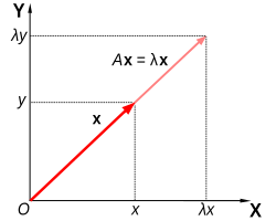
The eigenvectors v of this transformation satisfy equation (1), and the values of λ for which the determinant of the matrix (A − λI) equals zero are the eigenvalues.

The sum of the algebraic multiplicities of all distinct eigenvalues is μA = 4 = n, the order of the characteristic polynomial and the dimension of A.

Moreover, if the entire vector space V can be spanned by the eigenvectors of T, or equivalently if the direct sum of the eigenspaces associated with all the eigenvalues of T is the entire vector space V, then a basis of V called an eigenbasis can be formed from linearly independent eigenvectors of T. When T admits an eigenbasis, T is diagonalizable.

[43] Even for matrices whose elements are integers the calculation becomes nontrivial, because the sums are very long; the constant term is the determinant, which for an

Therefore, for matrices of order 5 or more, the eigenvalues and eigenvectors cannot be obtained by an explicit algebraic formula, and must therefore be computed by approximate numerical methods.

Efficient, accurate methods to compute eigenvalues and eigenvectors of arbitrary matrices were not known until the QR algorithm was designed in 1961.

[citation needed] For large Hermitian sparse matrices, the Lanczos algorithm is one example of an efficient iterative method to compute eigenvalues and eigenvectors, among several other possibilities.

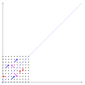
The eigendecomposition of a symmetric positive semidefinite (PSD) matrix yields an orthogonal basis of eigenvectors, each of which has a nonnegative eigenvalue.

Principal component analysis is used as a means of dimensionality reduction in the study of large data sets, such as those encountered in bioinformatics.

The principal eigenvector of a modified adjacency matrix of the World Wide Web graph gives the page ranks as its components.

The Perron–Frobenius theorem gives sufficient conditions for a Markov chain to have a unique dominant eigenvalue, which governs the convergence of the system to a steady state.

Eigenvalue problems occur naturally in the vibration analysis of mechanical structures with many degrees of freedom.

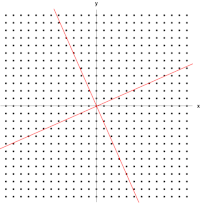
In mechanics, the eigenvectors of the moment of inertia tensor define the principal axes of a rigid body.

The tensor of moment of inertia is a key quantity required to determine the rotation of a rigid body around its center of mass.

Light, acoustic waves, and microwaves are randomly scattered numerous times when traversing a static disordered system.

In this case, the term eigenvector is used in a somewhat more general meaning, since the Fock operator is explicitly dependent on the orbitals and their eigenvalues.

In geology, especially in the study of glacial till, eigenvectors and eigenvalues are used as a method by which a mass of information of a clast's fabric can be summarized in a 3-D space by six numbers.

In the field, a geologist may collect such data for hundreds or thousands of clasts in a soil sample, which can be compared graphically or as a stereographic projection.

The eigenvectors of the covariance matrix associated with a large set of normalized pictures of faces are called eigenfaces; this is an example of principal component analysis.

In the facial recognition branch of biometrics, eigenfaces provide a means of applying data compression to faces for identification purposes.

Similar to this concept, eigenvoices represent the general direction of variability in human pronunciations of a particular utterance, such as a word in a language.