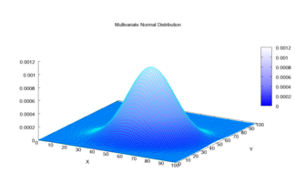
Multivariate normal distribution
The multivariate normal distribution is often used to describe, at least approximately, any set of (possibly) correlated real-valued random variables, each of which clusters around a mean value.
In the degenerate case where the covariance matrix is singular, the corresponding distribution has no density; see the section below for details.
This case arises frequently in statistics; for example, in the distribution of the vector of residuals in the ordinary least squares regression.
The circularly symmetric version of the complex normal distribution has a slightly different form.
To talk about densities but avoid dealing with measure-theoretic complications it can be simpler to restrict attention to a subset of
[9] To talk about densities meaningfully in singular cases, then, we must select a different base measure.
[10] The notion of cumulative distribution function (cdf) in dimension 1 can be extended in two ways to the multidimensional case, based on rectangular and ellipsoidal regions.
The interval for the multivariate normal distribution yields a region consisting of those vectors x satisfying Here
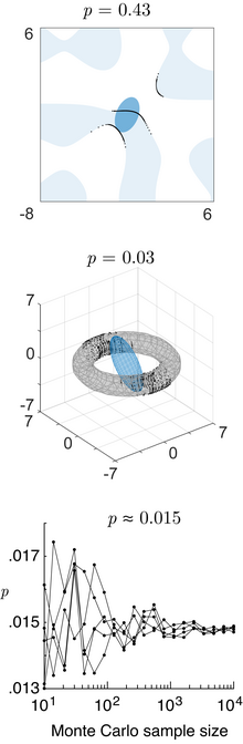
, then the ccdf can be written as a probability the maximum of dependent Gaussian variables:[15] While no simple closed formula exists for computing the ccdf, the maximum of dependent Gaussian variables can be estimated accurately via the Monte Carlo method.
is a scalar), which is relevant for Bayesian classification/decision theory using Gaussian discriminant analysis, is given by the generalized chi-squared distribution.
is a general function) can be computed using the numerical method of ray-tracing [17] (Matlab code).
That is, for a kth (= 2λ = 6) central moment, one sums the products of λ = 3 covariances (the expected value μ is taken to be 0 in the interests of parsimony): This yields
by the corresponding terms of the list consisting of r1 ones, then r2 twos, etc.. To illustrate this, examine the following 4th-order central moment case: where
With the above method one first finds the general case for a kth moment with k different X variables,
is simply the log of the probability density function: The circularly symmetric version of the noncentral complex case, where
, where the bars denote the matrix determinant, k is the dimensionality of the vector space, and the result has units of nats.
[citation needed] In general, random variables may be uncorrelated but statistically dependent.
But, as pointed out just above, it is not true that two random variables that are (separately, marginally) normally distributed and uncorrelated are independent.
matrix, then Y has a multivariate normal distribution with expected value c + Bμ and variance BΣBT i.e.,
This result follows by using Observe how the positive-definiteness of Σ implies that the variance of the dot product must be positive.
The equidensity contours of a non-singular multivariate normal distribution are ellipsoids (i.e. affine transformations of hyperspheres) centered at the mean.
If Σ = UΛUT = UΛ1/2(UΛ1/2)T is an eigendecomposition where the columns of U are unit eigenvectors and Λ is a diagonal matrix of the eigenvalues, then we have Moreover, U can be chosen to be a rotation matrix, as inverting an axis does not have any effect on N(0, Λ), but inverting a column changes the sign of U's determinant.
The distribution N(μ, Σ) is in effect N(0, I) scaled by Λ1/2, rotated by U and translated by μ. Conversely, any choice of μ, full rank matrix U, and positive diagonal entries Λi yields a non-singular multivariate normal distribution.
Geometrically this means that every contour ellipsoid is infinitely thin and has zero volume in n-dimensional space, as at least one of the principal axes has length of zero; this is the degenerate case.
is approximately 68.27%, but in higher dimensions the probability of finding a sample in the region of the standard deviation ellipse is lower.
[31] The derivation of the maximum-likelihood estimator of the covariance matrix of a multivariate normal distribution is straightforward.
[35] Mardia's test[36] is based on multivariate extensions of skewness and kurtosis measures.
Mardia's kurtosis statistic is skewed and converges very slowly to the limiting normal distribution.
, the parameters of the asymptotic distribution of the kurtosis statistic are modified[37] For small sample tests (
[41] Suppose that observations (which are vectors) are presumed to come from one of several multivariate normal distributions, with known means and covariances.