History of numerical weather prediction
The development of limited area (regional) models facilitated advances in forecasting the tracks of tropical cyclone as well as air quality in the 1970s and 1980s.
The MOS apply statistical techniques to post-process the output of dynamical models with the most recent surface observations and the forecast point's climatology.
Even with the increasing power of supercomputers, the forecast skill of numerical weather models only extends to about two weeks into the future, since the density and quality of observations—together with the chaotic nature of the partial differential equations used to calculate the forecast—introduce errors which double every five days.
In 1901 Cleveland Abbe, founder of the United States Weather Bureau, proposed that the atmosphere is governed by the same principles of thermodynamics and hydrodynamics that were studied in the previous century.
[2] He also identified seven variables that defined the state of the atmosphere at a given point: pressure, temperature, density, humidity, and the three components of the flow velocity vector.
Using a hydrostatic variation of Bjerknes's primitive equations,[2] Richardson produced by hand a 6-hour forecast for the state of the atmosphere over two points in central Europe, taking at least six weeks to do so.
[2] The first successful numerical prediction was performed using the ENIAC digital computer in 1950 by a team led by American meteorologist Jule Charney.
The team include Philip Thompson, Larry Gates, and Norwegian meteorologist Ragnar Fjørtoft, applied mathematician John von Neumann, and computer programmer Klara Dan von Neumann, M. H. Frankel, Jerome Namias, John C. Freeman Jr., Francis Reichelderfer, George Platzman, and Joseph Smagorinsky.
[8] In the United Kingdom the Meteorological Office first numerical weather prediction was completed by F. H. Bushby and Mavis Hinds in 1952 under the guidance of John Sawyer.
[10] In September 1954, Carl-Gustav Rossby assembled an international group of meteorologists in Stockholm and produced the first operational forecast (i.e. routine predictions for practical use) based on the barotropic equation.
[17] The first real-time forecasts made by Australia's Bureau of Meteorology in 1969 for portions of the Southern Hemisphere were also based on the single-layer barotropic model.
[19] Efforts to involve sea surface temperature in model initialization began in 1972 due to its role in modulating weather in higher latitudes of the Pacific.
[25] The United Kingdom Met Office has been running their global model since the late 1980s,[26] adding a 3D-Var data assimilation scheme in mid-1999.
[30] The GFS is slated to eventually be supplanted by the Flow-following, finite-volume Icosahedral Model (FIM), which like the GME is gridded on a truncated icosahedron, in the mid-2010s.
[33] The first general circulation climate model that combined both oceanic and atmospheric processes was developed in the late 1960s at the NOAA Geophysical Fluid Dynamics Laboratory.
[38] In comparison to traditional physics-based methods, machine learning (ML), or more broadly, artificial intelligence (AI) approaches, have demonstrated potential in enhancing weather forecasts (refer to the review by Shen et al.[39]).
As detailed in Table 4 of Shen et al., these AI-driven models were trained with ERA5 reanalysis data and CMIP6 datasets and evaluated using a variety of metrics such as root mean square errors (RMSE), anomaly correlation coefficients (ACC), Continuous Ranked Probability Score (CRPS), Temporal Anomaly Correlation Coefficient (TCC), Ranked Probability Skill Score (RPSS), Brier Skill Score (BSS), and bivariate correlation (COR).
By utilizing deep convolutional neural networks (CNNs), Weyn et al.[40] achieved lead times of 14 days.
In the third study, Bach et al. (2024)[43] utilized a hybrid dynamical and data-driven approach to show potential improvements in subseasonal monsoon prediction.
[54] Under the stimulus provided by the advent of stringent environmental control regulations, there was an immense growth in the use of air pollutant plume dispersion calculations between the late 1960s and today.
[55] In 1968, at a symposium sponsored by Conservation of Clean Air and Water in Europe, he compared many of the plume rise models then available in the literature.
[56] In that same year, Briggs also wrote the section of the publication edited by Slade[57] dealing with the comparative analyses of plume rise models.
Development of this model was taken over by the Environmental Protection Agency and improved in the mid to late 1970s using results from a regional air pollution study.
[62][63] The first operational air quality model in Canada, Canadian Hemispheric and Regional Ozone and NOx System (CHRONOS), began to be run in 2001.
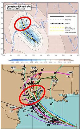
[66] In the early 1980s, the assimilation of satellite-derived winds from water vapor, infrared, and visible satellite imagery was found to improve tropical cyclones track forecasting.
[74] Since surface winds are the primary forcing mechanism in the spectral wave transport equation, ocean wave models use information produced by numerical weather prediction models as inputs to determine how much energy is transferred from the atmosphere into the layer at the surface of the ocean.
[75] Because forecast models based upon the equations for atmospheric dynamics do not perfectly determine weather conditions near the ground, statistical corrections were developed to attempt to resolve this problem.
[78] As proposed by Edward Lorenz in 1963, it is impossible for long-range forecasts—those made more than two weeks in advance—to predict the state of the atmosphere with any degree of skill, owing to the chaotic nature of the fluid dynamics equations involved.
Extremely small errors in temperature, winds, or other initial inputs given to numerical models will amplify and double every five days.
[79] Furthermore, existing observation networks have limited spatial and temporal resolution (for example, over large bodies of water such as the Pacific Ocean), which introduces uncertainty into the true initial state of the atmosphere.