Law of total variance

are random variables on the same probability space, and the variance of

In language perhaps better known to statisticians than to probability theorists, the two terms are the "unexplained" and the "explained" components of the variance respectively (cf.

fraction of variance unexplained, explained variation).

In actuarial science, specifically credibility theory, the first component is called the expected value of the process variance (EVPV) and the second is called the variance of the hypothetical means (VHM).

[3] These two components are also the source of the term "Eve's law", from the initials EV VE for "expectation of variance" and "variance of expectation".

To understand the formula above, we need to comprehend the random variables

is the variance of the expected values, i.e., it represents the part of the variance that is explained by the variation of the average value of

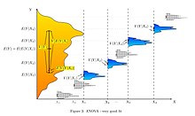
For an illustration, consider the example of a dog show (a selected excerpt of Analysis_of_variance#Example).

In this situation, it is reasonable to expect that the breed explains a major portion of the variance in weight since there is a big variance in the breeds' average weights.

Of course, there is still some variance in weight for each breed, which is taken into account in the "unexplained" term.

(e.g., for each breed in the example above) are very distinct, those variances are still combined in the "unexplained" term.

The data is summarized as follows: Among international students, the mean is

So the total variation is Suppose X is a coin flip with the probability of heads being h. Suppose that when X = heads then Y is drawn from a normal distribution with mean μh and standard deviation σh, and that when X = tails then Y is drawn from normal distribution with mean μt and standard deviation σt.

Then the first, "unexplained" term on the right-hand side of the above formula is the weighted average of the variances, hσh2 + (1 − h)σt2, and the second, "explained" term is the variance of the distribution that gives μh with probability h and gives μt with probability 1 − h. There is a general variance decomposition formula for

(this is where adherence to the conventional and rigidly case-sensitive notation of probability theory becomes important!).

Similar comments apply to the conditional variance.

One special case, (similar to the law of total expectation) states that if

is a partition of the whole outcome space, that is, these events are mutually exclusive and exhaustive, then

In this formula, the first component is the expectation of the conditional variance; the other two components are the variance of the conditional expectation.

Again, from the definition of variance, and applying the law of total expectation, we have

in terms of its variance and first moment, and apply the law of total expectation on the right hand side:

Finally, we recognize the terms in the second set of parentheses as the variance of the conditional expectation

The following formula shows how to apply the general, measure theoretic variance decomposition formula [4] to stochastic dynamic systems.

Suppose we have the internal histories (natural filtrations)

, each one corresponding to the history (trajectory) of a different collection of system variables.

It depends on the order of the conditioning in the sequential decomposition.

are such that the conditional expected value is linear; that is, in cases where

using data drawn from the joint distribution of

has a Gaussian distribution (and is an invertible function of

itself has a (marginal) Gaussian distribution, this explained component of variation sets a lower bound on the mutual information:[4]