Multivariate adaptive regression spline

In order to avoid trademark infringements, many open-source implementations of MARS are called "Earth".

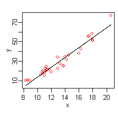
For example, the data could be: Here there is only one independent variable, so the x matrix is just a single column.

The figure on the right shows a plot of this function: a line giving the predicted

The data at the extremes of x indicates that the relationship between y and x may be non-linear (look at the red dots relative to the regression line at low and high values of x).

We thus turn to MARS to automatically build a model taking into account non-linearities.

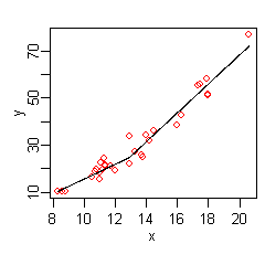
MARS software constructs a model from the given x and y as follows The figure on the right shows a plot of this function: the predicted

MARS has automatically produced a kink in the predicted y to take into account non-linearity.

In this simple example, we can easily see from the plot that y has a non-linear relationship with x (and might perhaps guess that y varies with the square of x).

The figure shows that wind does not affect the ozone level unless visibility is low.

We see that MARS can build quite flexible regression surfaces by combining hinge functions.

To obtain the above expression, the MARS model building procedure automatically selects which variables to use (some variables are important, others not), the positions of the kinks in the hinge functions, and how the hinge functions are combined.

For example, each line in the formula for ozone above is one basis function multiplied by its coefficient.

Examples of such basis functions can be seen in the middle three lines of the ozone formula.

A key part of MARS models are hinge functions taking the form or where

The figure on the right shows a mirrored pair of hinge functions with a knot at 3.1.

A hinge function is zero for part of its range, so can be used to partition the data into disjoint regions, each of which can be treated independently.

Thus for example a mirrored pair of hinge functions in the expression creates the piecewise linear graph shown for the simple MARS model in the previous section.

MARS builds a model in two phases: the forward and the backward pass.

MARS starts with a model which consists of just the intercept term (which is the mean of the response values).

MARS then repeatedly adds basis function in pairs to the model.

At each step it finds the pair of basis functions that gives the maximum reduction in sum-of-squares residual error (it is a greedy algorithm).

The maximum number of terms is specified by the user before model building starts.

Brute-force search can be sped up by using a heuristic that reduces the number of parent terms considered at each step ("Fast MARS"[4]).

Model subsets are compared using the Generalized cross validation (GCV) criterion described below.

The backward pass compares the performance of different models using Generalized Cross-Validation (GCV), a minor variant on the Akaike information criterion that approximates the leave-one-out cross-validation score in the special case where errors are Gaussian, or where the squared error loss function is used.

The effective number of parameters is defined as where penalty is typically 2 (giving results equivalent to the Akaike information criterion) but can be increased by the user if they so desire.

Thus the GCV formula adjusts (i.e. increases) the training RSS to penalize more complex models.

One constraint has already been mentioned: the user can specify the maximum number of terms in the forward pass.

A further constraint can be placed on the forward pass by specifying a maximum allowable degree of interaction.

Such constraints could make sense because of knowledge of the process that generated the data.