Perturbation (astronomy)
[2] The study of perturbations began with the first attempts to predict planetary motions in the sky.
Isaac Newton, at the time he formulated his laws of motion and of gravitation, applied them to the first analysis of perturbations,[2] recognizing the complex difficulties of their calculation.
[a] Many of the great mathematicians since then have given attention to the various problems involved; throughout the 18th and 19th centuries there was demand for accurate tables of the position of the Moon and planets for marine navigation.
This is called a two-body problem, or an unperturbed Keplerian orbit.
A general analytical solution (a mathematical expression to predict the positions and motions at any future time) exists for the two-body problem; when more than two bodies are considered analytic solutions exist only for special cases.
Even the two-body problem becomes insoluble if one of the bodies is irregular in shape.
In methods of general perturbations, general differential equations, either of motion or of change in the orbital elements, are solved analytically, usually by series expansions.
If all perturbations were to cease at any particular instant, the body would continue in this (now unchanging) conic section indefinitely; this conic is known as the osculating orbit and its orbital elements at any particular time are what are sought by the methods of general perturbations.
[2] General perturbations takes advantage of the fact that in many problems of celestial mechanics, the two-body orbit changes rather slowly due to the perturbations; the two-body orbit is a good first approximation.
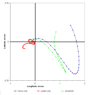
[6] In the Solar System, this is usually the case; Jupiter, the second largest body, has a mass of about 1/ 1000 that of the Sun.
General perturbation methods are preferred for some types of problems, as the source of certain observed motions are readily found.
This is not necessarily so for special perturbations; the motions would be predicted with similar accuracy, but no information on the configurations of the perturbing bodies (for instance, an orbital resonance) which caused them would be available.
[6] In methods of special perturbations, numerical datasets, representing values for the positions, velocities and accelerative forces on the bodies of interest, are made the basis of numerical integration of the differential equations of motion.
[6] Once applied only to comets and minor planets, special perturbation methods are now the basis of the most accurate machine-generated planetary ephemerides of the great astronomical almanacs.
and these are integrated numerically to form the new velocity and position vectors.
The advantage of Cowell's method is ease of application and programming.
Another disadvantage is that in systems with a dominant central body, such as the Sun, it is necessary to carry many significant digits in the arithmetic because of the large difference in the forces of the central body and the perturbing bodies, although with high precision numbers built into modern computers this is not as much of a limitation as it once was.
[12] Its advantages are that perturbations are generally small in magnitude, so the integration can proceed in larger steps (with resulting lesser errors), and the method is much less affected by extreme perturbations.
Its disadvantage is complexity; it cannot be used indefinitely without occasionally updating the osculating orbit and continuing from there, a process known as rectification.
Since the osculating orbit is easily calculated by two-body methods,
, is the difference of two nearly equal vectors, and further manipulation is necessary to avoid the need for extra significant digits.
This causes the bodies to follow motions that are periodic or quasi-periodic – such as the Moon in its strongly perturbed orbit, which is the subject of lunar theory.
This periodic nature led to the discovery of Neptune in 1846 as a result of its perturbations of the orbit of Uranus.
On-going mutual perturbations of the planets cause long-term quasi-periodic variations in their orbital elements, most apparent when two planets' orbital periods are nearly in sync.
This causes large perturbations of both, with a period of 918 years, the time required for the small difference in their positions at conjunction to make one complete circle, first discovered by Laplace.
In 25,000 years' time, Earth will have a more circular (less eccentric) orbit than Venus.
It has been shown that long-term periodic disturbances within the Solar System can become chaotic over very long time scales; under some circumstances one or more planets can cross the orbit of another, leading to collisions.
[c] The orbits of many of the minor bodies of the Solar System, such as comets, are often heavily perturbed, particularly by the gravitational fields of the gas giants.
While many of these perturbations are periodic, others are not, and these in particular may represent aspects of chaotic motion.
For example, in April 1996, Jupiter's gravitational influence caused the period of Comet Hale–Bopp's orbit to decrease from 4,206 to 2,380 years, a change that will not revert on any periodic basis.