Overfitting
[3]: 45 Underfitting occurs when a mathematical model cannot adequately capture the underlying structure of the data.
A function class that is too large, in a suitable sense, relative to the dataset size is likely to overfit.
To lessen the chance or amount of overfitting, several techniques are available (e.g., model comparison, cross-validation, regularization, early stopping, pruning, Bayesian priors, or dropout).
Burnham & Anderson, in their much-cited text on model selection, argue that to avoid overfitting, we should adhere to the "Principle of Parsimony".
Is the monkey who typed Hamlet actually a good writer?In regression analysis, overfitting occurs frequently.
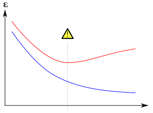
The goal is that the algorithm will also perform well on predicting the output when fed "validation data" that was not encountered during its training.
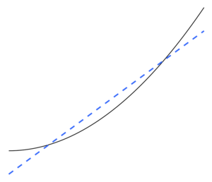
For an example where there are too many adjustable parameters, consider a dataset where training data for y can be adequately predicted by a linear function of two independent variables.
Everything else being equal, the more difficult a criterion is to predict (i.e., the higher its uncertainty), the more noise exists in past information that needs to be ignored.
Other negative consequences include: The optimal function usually needs verification on bigger or completely new datasets.
This matrix can be represented topologically as a complex network where direct and indirect influences between variables are visualized.
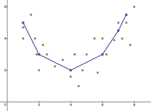
Underfitting is the inverse of overfitting, meaning that the statistical model or machine learning algorithm is too simplistic to accurately capture the patterns in the data.
In this case, bias in the parameter estimators is often substantial, and the sampling variance is underestimated, both factors resulting in poor confidence interval coverage.
Underfitted models tend to miss important treatment effects in experimental settings.There are multiple ways to deal with underfitting: Benign overfitting describes the phenomenon of a statistical model that seems to generalize well to unseen data, even when it has been fit perfectly on noisy training data (i.e., obtains perfect predictive accuracy on the training set).
The phenomenon is of particular interest in deep neural networks, but is studied from a theoretical perspective in the context of much simpler models, such as linear regression.
In other words, the number of directions in parameter space that are unimportant for prediction must significantly exceed the sample size.