Quantile-parameterized distribution
They were created to meet the need for easy-to-use continuous probability distributions flexible enough to represent a wide range of uncertainties, such as those commonly encountered in business, economics, engineering, and science.
Because QPDs are directly parameterized by data, they have the practical advantage of avoiding the intermediate step of parameter estimation, a time-consuming process that typically requires non-linear iterative methods to estimate probability-distribution parameters from data.
Some QPDs have virtually unlimited shape flexibility and closed-form moments as well.
Historically, the Pearson[1] and Johnson[2][3] families of distributions have been used when shape flexibility is needed.
That is because both families can match the first four moments (mean, variance, skewness, and kurtosis) of any data set.
However, if the characteristics of this population are such that the desired cumulative distribution function (CDF) should run through certain specific CDF points, there may be no beta distribution that meets this need.
Because the beta distribution has only two shape parameters, it cannot, in general, match even three specified CDF points.
Moreover, the beta parameters that best fit such data can be found only by nonlinear iterative methods.
Practitioners of decision analysis, needing distributions easily parameterized by three or more CDF points (e.g., because such points were specified as the result of an expert-elicitation process), originally invented quantile-parameterized distributions for this purpose.
Subsequently, Keelin (2016)[5] developed the metalog distributions, a family of quantile-parameterized distributions that has virtually unlimited shape flexibility, simple equations, and closed-form moments.
are continuously differentiable and linearly independent basis functions.
are the lower and upper bounds (if they exist) of a random variable with quantile function
These distributions are called quantile-parameterized because for a given set of quantile pairs
[4] If one desires to use more quantile pairs than basis functions, then the coefficients
can be chosen to minimize the sum of squared errors between the stated quantiles
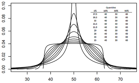
Some skewed and symmetric Simple Q-Normal PDFs are shown in the figures below.
Note that this PDF is expressed as a function of cumulative probability
An alternate method, implemented as a linear program, determines the coefficients by minimizing the sum of absolute distances between the CDF and the data subject to feasibility constraints.
is the quantile function of the lognormal distribution with lower bound
Similarly, applying this log transformation to the unbounded metalog distribution[9] yields the semi-bounded (log) metalog distribution;[10] likewise, applying the logit transformation,
is any QPD that meets Keelin and Powley’s definition, the transformed variable maintains the above properties of feasibility, convexity, and fitting to data.
Moreover, such transformed QPDs share the same set of feasible coefficients as the underlying untransformed QPD.
is expressed in closed form, Keelin and Powley QPDs facilitate Monte Carlo simulation.
in closed form, thereby eliminating the need to invert a CDF expressed as
JQPDs do not meet Keelin and Powley’s QPD definition, but rather have their own properties.
JQPDs are feasible for all SPT parameter sets that are consistent with the rules of probability.
The original applications of QPDs were by decision analysts wishing to conveniently convert expert-assessed quantiles (e.g., 10th, 50th, and 90th quantiles) into smooth continuous probability distributions.
Similarly, since QPDs can impose fewer shape constraints than traditional distributions, they have been used to fit a wide range of empirical data in order to represent those data sets as continuous distributions (e.g., reflecting bimodality that may exist in the data in a straightforward manner[17]).
Keelin et al. (2019)[18] apply this to the sum of independent identically distributed lognormal distributions, where quantiles of the sum can be determined by a large number of simulations.
QPDs have also been applied to assess the risks of asteroid impact,[19] cybersecurity,[6][20] biases in projections of oil-field production when compared to observed production after the fact,[21] and future Canadian population projections based on combining the probabilistic views of multiple experts.