Time–temperature superposition
[5] The application of the principle typically involves the following steps: The translation factor is often computed using an empirical relation first established by Malcolm L. Williams, Robert F. Landel and John D. Ferry (also called the Williams-Landel-Ferry or WLF model).
Some materials, polymers in particular, show a strong dependence of viscoelastic properties on the temperature at which they are measured.
If you plot the elastic modulus of a noncrystallizing crosslinked polymer against the temperature at which you measured it, you will get a curve which can be divided up into distinct regions of physical behavior.
At very low temperatures, the polymer will behave like a glass and exhibit a high modulus.
In the 1940s Andrews and Tobolsky[6] showed that there was a simple relationship between temperature and time for the mechanical response of a polymer.
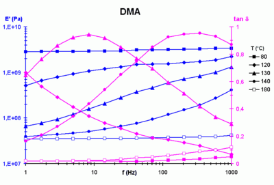
Modulus measurements are made by stretching or compressing a sample at a prescribed rate of deformation.
For polymers, changing the rate of deformation will cause the curve described above to be shifted along the temperature axis.
It has been shown experimentally that the elastic modulus (E) of a polymer is influenced by the load and the response time.
Time–temperature superposition is a procedure that has become important in the field of polymers to observe the dependence upon temperature on the change of viscosity of a polymeric fluid.
Time–temperature superposition avoids the inefficiency of measuring a polymer's behavior over long periods of time at a specified temperature by utilizing the fact that at higher temperatures and shorter time the polymer will behave the same, provided there are no phase transitions.
In other words, The quantity aT is called the horizontal translation factor or the shift factor and has the properties: The superposition principle for complex dynamic moduli (G* = G' + i G'' ) at a fixed frequency ω is obtained similarly: A decrease in temperature increases the time characteristics while frequency characteristics decrease.
For a polymer in solution or "molten" state the following relationship can be used to determine the shift factor: where ηT0 is the viscosity (non-Newtonian) during continuous flow at temperature T0 and ηT is the viscosity at temperature T. The time–temperature shift factor can also be described in terms of the activation energy (Ea).
By plotting the shift factor aT versus the reciprocal of temperature (in K), the slope of the curve can be interpreted as Ea/k, where k is the Boltzmann constant = 8.64x10⁻⁵ eV/K and the activation energy is expressed in terms of eV.
is the decadic logarithm and C1 and C2 are positive constants that depend on the material and the reference temperature.
A good correlation between the two shift factors gives the values of the coefficients C1 and C2 that characterize the material.
These orders of magnitude are useful and are a good indicator of the quality of a relationship that has been computed from experimental data.
The principle of time-temperature superposition requires the assumption of thermorheologically simple behavior (all curves have the same characteristic time variation law with temperature).
This amounts to explore a part of the master curve corresponding to frequencies lower than ω1 while maintaining the temperature at T0.
The viscoelastic behavior is well modeled and allows extrapolation beyond the field of experimental frequencies which typically ranges from 0.01 to 100 Hz .
The WLF-model can be developed from Doolittle's concept of free volume and the thermal expansion coefficient
The study to determine aT and the coefficients C1 and C2 requires extensive dynamic testing at a number of scanning frequencies and temperature, which represents at least a hundred measurement points.