Indifference curve
One can also refer to each point on the indifference curve as rendering the same level of utility (satisfaction) for the consumer.
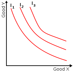
In other words, an indifference curve is the locus of various points showing different combinations of two goods providing equal utility to the consumer.
[1] The main use of indifference curves is in the representation of potentially observable demand patterns for individual consumers over commodity bundles.
The slope of an indifference curve is called the MRS (marginal rate of substitution), and it indicates how much of good y must be sacrificed to keep the utility constant if good x is increased by one unit.
If the marginal rate of substitution is diminishing along an indifference curve, that is the magnitude of the slope is decreasing or becoming less steep, then the preference is convex.
The theory of indifference curves was developed by Francis Ysidro Edgeworth, who explained in his 1881 book the mathematics needed for their drawing;[3] later on, Vilfredo Pareto was the first author to actually draw these curves, in his 1906 book.
[4][5] The theory can be derived from William Stanley Jevons' ordinal utility theory, which posits that individuals can always rank any consumption bundles by order of preference.
If you move "off" an indifference curve traveling in a northeast direction (assuming positive marginal utility for the goods) you are essentially climbing a mound of utility.
The non-satiation requirement means that you will never reach the "top," or a "bliss point," a consumption bundle that is preferred to all others.
Indifference curves are typically[vague] represented[clarification needed] to be: It also implies that the commodities are good rather than bad.
Budget constraints give a straight line on the indifference map showing all the possible distributions between the two goods; the point of maximum utility is then the point at which an indifference curve is tangent to the budget line (illustrated).
The process then continues until the market's and household's marginal rates of substitution are equal.
[10] Now, if the price of carrots were to change, and the price of all other goods were to remain constant, the gradient of the budget line would also change, leading to a different point of tangency and a different quantity demanded.
These price / quantity combinations can then be used to deduce a full demand curve.
The line connecting all points of tangency between the indifference curve and the budget constraint as the budget constraint changes is called the expansion path,[11] and correlates to shifts in demand.
The slope of an indifference curve (in absolute value), known by economists as the marginal rate of substitution, shows the rate at which consumers are willing to give up one good in exchange for more of the other good.
The curves are convex to the origin, describing the negative substitution effect.
As price rises for a fixed money income, the consumer seeks the less expensive substitute at a lower indifference curve.
The negative slope of the indifference curve incorporates the willingness of the consumer to make trade offs.
[9] If two goods are perfect substitutes then the indifference curves will have a constant slope since the consumer would be willing to switch between at a fixed ratio.
, meaning not that they are unwanted but that they are equally good in satisfying preferences.
In utility theory, the utility function of an agent is a function that ranks all pairs of consumption bundles by order of preference (completeness) such that any set of three or more bundles forms a transitive relation.
such that, in the end, there is no change in U: Thus, the ratio of marginal utilities gives the absolute value of the slope of the indifference curve at point
The marginal utilities are given by and Therefore, along an indifference curve, These examples might be useful for modelling individual or aggregate demand.
As used in biology, the indifference curve is a model for how animals 'decide' whether to perform a particular behavior, based on changes in two variables which can increase in intensity, one along the x-axis and the other along the y-axis.
The indifference curve is drawn to predict the animal's behavior at various levels of risk and food availability.
Indifference curves inherit the criticisms directed at utility more generally.
He argues that the presence of an endowment effect indicates that a person has no indifference curve (see however Hanemann, 1991[14]) rendering the neoclassical tools of welfare analysis useless, concluding that courts should instead use WTA as a measure of value.
Fischel (1995)[15] however, raises the counterpoint that using WTA as a measure of value would deter the development of a nation's infrastructure and economic growth.
Austrian economist Murray Rothbard criticised the indifference curve as "never by definition exhibited in action, in actual exchanges, and is therefore unknowable and objectively meaningless.