Cumulative distribution function
In probability theory and statistics, the cumulative distribution function (CDF) of a real-valued random variable
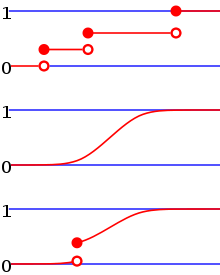
[1] Every probability distribution supported on the real numbers, discrete or "mixed" as well as continuous, is uniquely identified by a right-continuous monotone increasing function (a càdlàg function)
In the case of a scalar continuous distribution, it gives the area under the probability density function from negative infinity to
The cumulative distribution function of a real-valued random variable
is the function given by[2]: p. 77 where the right-hand side represents the probability that the random variable
, is therefore[2]: p. 84 In the definition above, the "less than or equal to" sign, "≤", is a convention, not a universally used one (e.g. Hungarian literature uses "<"), but the distinction is important for discrete distributions.
The proper use of tables of the binomial and Poisson distributions depends upon this convention.
The probability density function of a continuous random variable can be determined from the cumulative distribution function by differentiating[3] using the Fundamental Theorem of Calculus; i.e. given
is a purely discrete random variable, then it attains values
as shown in the diagram (consider the areas of the two red rectangles and their extensions to the right or left up to the graph of
In addition, the (finite) expected value of the real-valued random variable
can be defined on the graph of its cumulative distribution function as illustrated by the drawing in the definition of expected value for arbitrary real-valued random variables.
Sometimes, it is useful to study the opposite question and ask how often the random variable is above a particular level.
This has applications in statistical hypothesis testing, for example, because the one-sided p-value is the probability of observing a test statistic at least as extreme as the one observed.
Thus, provided that the test statistic, T, has a continuous distribution, the one-sided p-value is simply given by the ccdf: for an observed value
often has an S-like shape, an alternative illustration is the folded cumulative distribution or mountain plot, which folds the top half of the graph over,[5][6] that is where
This form of illustration emphasises the median, dispersion (specifically, the mean absolute deviation from the median[7]) and skewness of the distribution or of the empirical results.
A number of results exist to quantify the rate of convergence of the empirical distribution function to the underlying cumulative distribution function.
[9] When dealing simultaneously with more than one random variable the joint cumulative distribution function can also be defined.
is given by[2]: p. 89 where the right-hand side represents the probability that the random variable
Example of joint cumulative distribution function: For two continuous variables X and Y:
For two discrete random variables, it is beneficial to generate a table of probabilities and address the cumulative probability for each potential range of X and Y, and here is the example:[10] given the joint probability mass function in tabular form, determine the joint cumulative distribution function.
Solution: using the given table of probabilities for each potential range of X and Y, the joint cumulative distribution function may be constructed in tabular form: For
The probability that a point belongs to a hyperrectangle is analogous to the 1-dimensional case:[11]
The generalization of the cumulative distribution function from real to complex random variables is not obvious because expressions of the form
The concept of the cumulative distribution function makes an explicit appearance in statistical analysis in two (similar) ways.
The empirical distribution function is a formal direct estimate of the cumulative distribution function for which simple statistical properties can be derived and which can form the basis of various statistical hypothesis tests.
Such tests can assess whether there is evidence against a sample of data having arisen from a given distribution, or evidence against two samples of data having arisen from the same (unknown) population distribution.
The closely related Kuiper's test is useful if the domain of the distribution is cyclic as in day of the week.
For instance Kuiper's test might be used to see if the number of tornadoes varies during the year or if sales of a product vary by day of the week or day of the month.