Pole splitting
Pole splitting is a phenomenon exploited in some forms of frequency compensation used in an electronic amplifier.
This pole movement increases the stability of the amplifier and improves its step response at the cost of decreased speed.
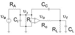
[5] The amplifier of Figure 1 has a low frequency pole due to the added input resistance Ri and capacitance Ci, with the time constant Ci ( RA || Ri ).
The amplifier is given a high frequency output pole by addition of the load resistance RL and capacitance CL, with the time constant CL ( Ro || RL ).
The upward movement of the high-frequency pole occurs because the Miller-amplified compensation capacitor CC alters the frequency dependence of the output voltage divider.
The first objective, to show the lowest pole moves down in frequency, is established using the same approach as the Miller's theorem article.
to the ideal op amp as a function of the applied signal voltage
, namely, which exhibits a roll-off with frequency beginning at f1 where which introduces notation
Turning to the second objective, showing the higher pole moves still higher in frequency, it is necessary to look at the output side of the circuit, which contributes a second factor to the overall gain, and additional frequency dependence.
is determined by the gain of the ideal op amp inside the amplifier as Using this relation and applying Kirchhoff's current law to the output side of the circuit determines the load voltage
at the input to the ideal op amp as: This expression is combined with the gain factor found earlier for the input side of the circuit to obtain the overall gain as This gain formula appears to show a simple two-pole response with two time constants.
(It also exhibits a zero in the numerator but, assuming the amplifier gain Av is large, this zero is important only at frequencies too high to matter in this discussion, so the numerator can be approximated as unity.)
That is, assuming the output R-C product, CL ( Ro || RL ), corresponds to a frequency well above the low frequency pole, the accurate form of the Miller capacitance must be used, rather than the Miller approximation.
Upon substitution of this result into the gain expression and collecting terms, the gain is rewritten as: with Dω given by a quadratic in ω, namely: Every quadratic has two factors, and this expression looks simpler if it is rewritten as where
is the longest time constant, corresponding to the lowest pole, and suppose
At low frequencies near the lowest pole of this amplifier, ordinarily the linear term in ω is more important than the quadratic term, so the low frequency behavior of Dω is: where now CM is redefined using the Miller approximation as
which is simply the previous Miller capacitance evaluated at low frequencies.
is much larger than its original value of Ci ( RA || Ri ).
is valid, the second time constant, the position of the high frequency pole, is found from the quadratic term in Dω as Substituting in this expression the quadratic coefficient corresponding to the product
, an estimate for the position of the second pole is found: and because CM is large, it seems
For general purpose use, traditional design (often called dominant-pole or single-pole compensation) requires the amplifier gain to drop at 20 dB/decade from the corner frequency down to 0 dB gain, or even lower.
[9] [10] With this design the amplifier is stable and has near-optimal step response even as a unity gain voltage buffer.
At the lowest pole f1, the Bode gain plot breaks slope to fall at 20 dB/decade.
The aim is to maintain the 20 dB/decade slope all the way down to zero dB, and taking the ratio of the desired drop in gain (in dB) of 20 log10 Av to the required change in frequency (on a log frequency scale[13]) of ( log10 f2 − log10 f1 ) = log10 ( f2 / f1 ) the slope of the segment between f1 and f2 is: which is 20 dB/decade provided f2 = Av f1 .
If f2 is not this large, the second break in the Bode plot that occurs at the second pole interrupts the plot before the gain drops to 0 dB with consequent lower stability and degraded step response.
Figure 3 shows that to obtain the correct gain dependence on frequency, the second pole is at least a factor Av higher in frequency than the first pole.
The gain is reduced a bit by the voltage dividers at the input and output of the amplifier, so with corrections to Av for the voltage dividers at input and output the pole-ratio condition for good step response becomes: Using the approximations for the time constants developed above, or which provides a quadratic equation to determine an appropriate value for CC.
However, when large signals are used, the need to charge and discharge the compensation capacitor adversely affects the amplifier slew rate; in particular, the response to an input ramp signal is limited by the need to charge CC.