Simple linear regression

The adjective simple refers to the fact that the outcome variable is related to a single predictor.

In this case, the slope of the fitted line is equal to the correlation between y and x corrected by the ratio of standard deviations of these variables.

Consider the model function which describes a line with slope β and y-intercept α.

Suppose we observe n data pairs and call them {(xi, yi), i = 1, ..., n}.

We can describe the underlying relationship between yi and xi involving this error term εi by This relationship between the true (but unobserved) underlying parameters α and β and the data points is called a linear regression model.

for the parameters α and β which would provide the "best" fit in some sense for the data points.

solve the following minimization problem: where the objective function Q is: By expanding to get a quadratic expression in

For example: This notation allows us a concise formula for rxy: The coefficient of determination ("R squared") is equal to

(thereby not changing it): We can see that the slope (tangent of angle) of the regression line is the weighted average of

This assumption is used when deriving the standard error of the slope and showing that it is unbiased.

is not actually a random variable, what type of parameter does the empirical correlation

defines a random variable drawn from the empirical distribution of the x values in our sample.

For example, if x had 10 values from the natural numbers: [1,2,3...,10], then we can imagine x to be a Discrete uniform distribution.

The following is based on assuming the validity of a model under which the estimates are optimal.

We consider the residuals εi as random variables drawn independently from some distribution with mean zero.

will themselves be random variables whose means will equal the "true values" α and β.

The variance of the mean response is given by:[11] This expression can be simplified to where m is the number of data points.

(a fixed but unknown parameter that can be estimated), the variance of the predicted response is given by

The formulas given in the previous section allow one to calculate the point estimates of α and β — that is, the coefficients of the regression line for the given set of data.

Confidence intervals were devised to give a plausible set of values to the estimates one might have if one repeated the experiment a very large number of times.

where σ2 is the variance of the error terms (see Proofs involving ordinary least squares).

At the same time the sum of squared residuals Q is distributed proportionally to χ2 with n − 2 degrees of freedom, and independently from

The alternative second assumption states that when the number of points in the dataset is "large enough", the law of large numbers and the central limit theorem become applicable, and then the distribution of the estimators is approximately normal.

Under this assumption all formulas derived in the previous section remain valid, with the only exception that the quantile t*n−2 of Student's t distribution is replaced with the quantile q* of the standard normal distribution.

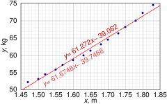
The 0.975 quantile of Student's t-distribution with 13 degrees of freedom is t*13 = 2.1604, and thus the 95% confidence intervals for α and β are The product-moment correlation coefficient might also be calculated: In SLR, there is an underlying assumption that only the dependent variable contains measurement error; if the explanatory variable is also measured with error, then simple regression is not appropriate for estimating the underlying relationship because it will be biased due to regression dilution.

Other estimation methods that can be used in place of ordinary least squares include least absolute deviations (minimizing the sum of absolute values of residuals) and the Theil–Sen estimator (which chooses a line whose slope is the median of the slopes determined by pairs of sample points).

Deming regression (total least squares) also finds a line that fits a set of two-dimensional sample points, but (unlike ordinary least squares, least absolute deviations, and median slope regression) it is not really an instance of simple linear regression, because it does not separate the coordinates into one dependent and one independent variable and could potentially return a vertical line as its fit.

Several methods exist, considering: Sometimes it is appropriate to force the regression line to pass through the origin, because x and y are assumed to be proportional.

For the model without the intercept term, y = βx, the OLS estimator for β simplifies to Substituting (x − h, y − k) in place of (x, y) gives the regression through (h, k): where Cov and Var refer to the covariance and variance of the sample data (uncorrected for bias).

The last form above demonstrates how moving the line away from the center of mass of the data points affects the slope.