Skewness

For example, a zero value in skewness means that the tails on both sides of the mean balance out overall; this is the case for a symmetric distribution but can also be true for an asymmetric distribution where one tail is long and thin, and the other is short but fat.

These tapering sides are called tails, and they provide a visual means to determine which of the two kinds of skewness a distribution has: Skewness in a data series may sometimes be observed not only graphically but by simple inspection of the values.

[3] If the distribution is both symmetric and unimodal, then the mean = median = mode.

Note, however, that the converse is not true in general, i.e. zero skewness (defined below) does not imply that the mean is equal to the median.

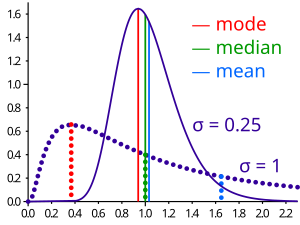
A 2005 journal article points out:[2]Many textbooks teach a rule of thumb stating that the mean is right of the median under right skew, and left of the median under left skew.

Most commonly, though, the rule fails in discrete distributions where the areas to the left and right of the median are not equal.

Such distributions not only contradict the textbook relationship between mean, median, and skew, they also contradict the textbook interpretation of the median.For example, in the distribution of adult residents across US households, the skew is to the right.

However, since the majority of cases is less than or equal to the mode, which is also the median, the mean sits in the heavier left tail.

As a result, the rule of thumb that the mean is right of the median under right skew failed.

, defined as:[4][5] where μ is the mean, σ is the standard deviation, E is the expectation operator, μ3 is the third central moment, and κt are the t-th cumulants.

If σ is finite and μ is finite too, then skewness can be expressed in terms of the non-central moment E[X3] by expanding the previous formula: Skewness can be infinite, as when where the third cumulants are infinite, or as when where the third cumulant is undefined.

For a sample of n values, two natural estimators of the population skewness are[6] and where

is the version found in Excel and several statistical packages including Minitab, SAS and SPSS.

; their expected values can even have the opposite sign from the true skewness.

For instance, a mixed distribution consisting of very thin Gaussians centred at −99, 0.5, and 2 with weights 0.01, 0.66, and 0.33 has a skewness

has an expected value of about 0.32, since usually all three samples are in the positive-valued part of the distribution, which is skewed the other way.

Skewness is a descriptive statistic that can be used in conjunction with the histogram and the normal quantile plot to characterize the data or distribution.

With pronounced skewness, standard statistical inference procedures such as a confidence interval for a mean will be not only incorrect, in the sense that the true coverage level will differ from the nominal (e.g., 95%) level, but they will also result in unequal error probabilities on each side.

Skewness can be used to obtain approximate probabilities and quantiles of distributions (such as value at risk in finance) via the Cornish–Fisher expansion.

Many models assume normal distribution; i.e., data are symmetric about the mean.

So, an understanding of the skewness of the dataset indicates whether deviations from the mean are going to be positive or negative.

, which for symmetric distributions is equal to the MAD measure of dispersion.

This definition leads to a corresponding overall measure of skewness[23] defined as the supremum of this over the range 1/2 ≤ u < 1.

[22] Quantile-based skewness measures are at first glance easy to interpret, but they often show significantly larger sample variations than moment-based methods.

Groeneveld and Meeden have suggested, as an alternative measure of skewness,[22] where μ is the mean, ν is the median, |...| is the absolute value, and E() is the expectation operator.

This is closely related in form to Pearson's second skewness coefficient.

Use of L-moments in place of moments provides a measure of skewness known as the L-skewness.

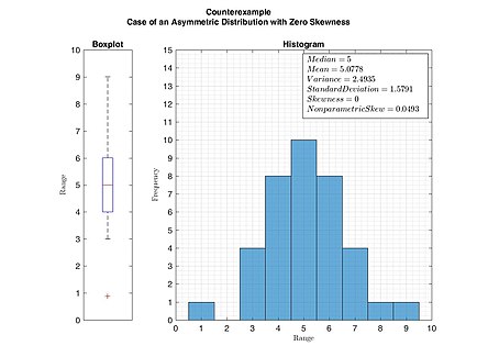
[25] A value of skewness equal to zero does not imply that the probability distribution is symmetric.

If X is a random variable taking values in the d-dimensional Euclidean space, X has finite expectation, X' is an independent identically distributed copy of X, and

[27] Thus there is a simple consistent statistical test of diagonal symmetry based on the sample distance skewness: The medcouple is a scale-invariant robust measure of skewness, with a breakdown point of 25%.