Algorithmic inference

Algorithmic inference gathers new developments in the statistical inference methods made feasible by the powerful computing devices widely available to any data analyst.

The main focus is on the algorithms which compute statistics rooting the study of a random phenomenon, along with the amount of data they must feed on to produce reliable results.

This shifts the interest of mathematicians from the study of the distribution laws to the functional properties of the statistics, and the interest of computer scientists from the algorithms for processing data to the information they process.

Concerning the identification of the parameters of a distribution law, the mature reader may recall lengthy disputes in the mid 20th century about the interpretation of their variability in terms of fiducial distribution (Fisher 1956), structural probabilities (Fraser 1966), priors/posteriors (Ramsey 1925), and so on.

From an epistemology viewpoint, this entailed a companion dispute as to the nature of probability: is it a physical feature of phenomena to be described through random variables or a way of synthesizing data about a phenomenon?

Opting for the latter, Fisher defines a fiducial distribution law of parameters of a given random variable that he deduces from a sample of its specifications.

Fisher fought hard to defend the difference and superiority of his notion of parameter distribution in comparison to analogous notions, such as Bayes' posterior distribution, Fraser's constructive probability and Neyman's confidence intervals.

For half a century, Neyman's confidence intervals won out for all practical purposes, crediting the phenomenological nature of probability.

Because of their randomness, you may compute from the sample specific intervals containing the fixed μ with a given probability that you denote confidence.

Working with statistics and is the sample mean, we recognize that follows a Student's t distribution (Wilks 1962) with parameter (degrees of freedom) m − 1, so that Gauging T between two quantiles and inverting its expression as a function of

From a modeling perspective the entire dispute looks like a chicken-egg dilemma: either fixed data by first and probability distribution of their properties as a consequence, or fixed properties by first and probability distribution of the observed data as a corollary.

Per se, the task of computing a Neyman confidence interval for the fixed parameter θ is hard: you do not know θ, but you look for disposing around it an interval with a possibly very low probability of failing.

The analytical solution is allowed for a very limited number of theoretical cases.

Vice versa a large variety of instances may be quickly solved in an approximate way via the central limit theorem in terms of confidence interval around a Gaussian distribution – that's the benefit.

The drawback is that the central limit theorem is applicable when the sample size is sufficiently large.

Rather, this size is not sufficiently large because of the complexity of the inference problem.

With the availability of large computing facilities, scientists refocused from isolated parameters inference to complex functions inference, i.e. re sets of highly nested parameters identifying functions.

In these cases we speak about learning of functions (in terms for instance of regression, neuro-fuzzy system or computational learning) on the basis of highly informative samples.

Focusing on the sample size ensuring a limited learning error with a given confidence level, the consequence is that the lower bound on this size grows with complexity indices such as VC dimension or detail of a class to which the function we want to learn belongs.

A sample of 1,000 independent bits is enough to ensure an absolute error of at most 0.081 on the estimation of the parameter p of the underlying Bernoulli variable with a confidence of at least 0.99.

The same size cannot guarantee a threshold less than 0.088 with the same confidence 0.99 when the error is identified with the probability that a 20-year-old man living in New York does not fit the ranges of height, weight and waistline observed on 1,000 Big Apple inhabitants.

The accuracy shortage occurs because both the VC dimension and the detail of the class of parallelepipeds, among which the one observed from the 1,000 inhabitants' ranges falls, are equal to 6.

In order to ensure this population clean properties, it is enough to draw randomly the seed values and involve either sufficient statistics or, simply, well-behaved statistics w.r.t.

derived from a master equation rooted on a well-behaved statistic s. You may find the distribution law of the Pareto parameters A and K as an implementation example of the population bootstrap method as in the figure on the left.

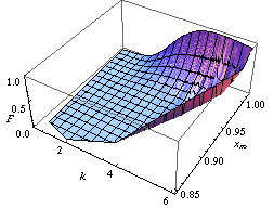
Computing a confidence interval for M given its distribution function is straightforward: we need only find two quantiles (for instance

quantiles in case we are interested in a confidence interval of level δ symmetric in the tail's probabilities) as indicated on the left in the diagram showing the behavior of the two bounds for different values of the statistic sm.

On the contrary, with the last approach (and above-mentioned methods: population bootstrap and twisting argument) we may learn the joint distribution of many parameters.

The former concerns the probability with which an extended support vector machine attributes a binary label 1 to the points of the

The two surfaces are drawn on the basis of a set of sample points in turn labelled according to a specific distribution law (Apolloni et al. 2008).

The latter concerns the confidence region of the hazard rate of breast cancer recurrence computed from a censored sample (Apolloni, Malchiodi & Gaito 2006).