Confidence interval
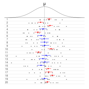
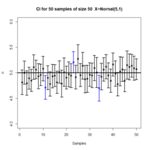
More specifically, a CI is a random interval which contains the parameter being estimated at a given percentage of the time (under replication).
Sometimes one has to make do with approximations, hence the confidence level is only approximate[3] Factors affecting the width of the CI include the sample size, the variability in the sample, and the confidence level.
[5] Methods for calculating confidence intervals for the binomial proportion appeared from the 1920s.
[11] Neyman described the development of the ideas as follows (reference numbers have been changed):[10] [My work on confidence intervals] originated about 1930 from a simple question of Waclaw Pytkowski, then my student in Warsaw, engaged in an empirical study in farm economics.
The question was: how to characterize non-dogmatically the precision of an estimated regression coefficient?
Quite unexpectedly, while the conceptual framework of fiducial argument is entirely different from that of confidence intervals, the specific solutions of several particular problems coincided.
Thus, in the first paper in which I presented the theory of confidence intervals, published in 1934,[8] I recognized Fisher's priority for the idea that interval estimation is possible without any reference to Bayes' theorem and with the solution being independent from probabilities a priori.
At the same time I mildly suggested that Fisher's approach to the problem involved a minor misunderstanding.
Alternatively, some authors[16] simply require that which is useful if the probabilities are only partially identified or imprecise, and also when dealing with discrete distributions.
These will have been devised so as to meet certain desirable properties, which will hold given that the assumptions on which the procedure relies are true.
This means that the rule for constructing the confidence interval should make as much use of the information in the data-set as possible.
For example, a survey might result in an estimate of the median income in a population, but it might equally be considered as providing an estimate of the logarithm of the median income, given that this is a common scale for presenting graphical results.
For non-standard applications, there are several routes that might be taken to derive a rule for the construction of confidence intervals.
Established rules for standard procedures might be justified or explained via several of these routes.
Typically a rule for constructing confidence intervals is closely tied to a particular way of finding a point estimate of the quantity being considered.
The central limit theorem is a refinement of the law of large numbers.
For a large number of independent identically distributed random variables
is an independent sample from a normally distributed population with unknown parameters mean
Confidence intervals and levels are frequently misunderstood, and published studies have shown that even professional scientists often misinterpret them.
[21][22][23][24][25][26] It will be noticed that in the above description, the probability statements refer to the problems of estimation with which the statistician will be concerned in the future.
In fact, I have repeatedly stated that the frequency of correct results will tend to α.
Can we say that in this particular case the probability of the true value [falling between these limits] is equal to α?
Robinson[30] called this example "[p]ossibly the best known counterexample for Neyman's version of confidence interval theory."
is[31] A fiducial or objective Bayesian argument can be used to derive the interval estimate which is also a 50% confidence procedure.
: Therefore, the nominal 50% confidence coefficient is unrelated to the uncertainty we should have that a specific interval contains the true value.
Yet the first interval will exclude almost all reasonable values of the parameter due to its short width.
Steiger[32] suggested a number of confidence procedures for common effect size measures in ANOVA.
Morey et al.[27] point out that several of these confidence procedures, including the one for ω2, have the property that as the F statistic becomes increasingly small—indicating misfit with all possible values of ω2—the confidence interval shrinks and can even contain only the single value ω2 = 0; that is, the CI is infinitesimally narrow (this occurs when
This behavior is consistent with the relationship between the confidence procedure and significance testing: as F becomes so small that the group means are much closer together than we would expect by chance, a significance test might indicate rejection for most or all values of ω2.
This is contrary to the common interpretation of confidence intervals that they reveal the precision of the estimate.