Factorial experiment

A 2x2 factorial design, for instance, has two factors, each with two levels, leading to four unique combinations to test.

This method strategically omits some combinations (usually at least half) to make the experiment more manageable.

Factorial designs were used in the 19th century by John Bennet Lawes and Joseph Henry Gilbert of the Rothamsted Experimental Station.

Nature, he suggests, will best respond to a logical and carefully thought out questionnaire; indeed, if we ask her a single question, she will often refuse to answer until some other topic has been discussed.

Compared to such one-factor-at-a-time (OFAT) experiments, factorial experiments offer several advantages[4][5] The main disadvantage of the full factorial design is its sample size requirement, which grows exponentially with the number of factors or inputs considered.

In his book, Improving Almost Anything: Ideas and Essays, statistician George Box gives many examples of the benefits of factorial experiments.

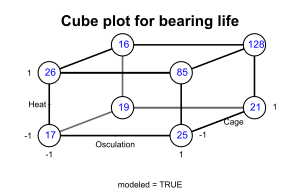
Christer showed them how they could test two additional factors "for free" – without increasing the number of runs and without reducing the accuracy of their estimate of the cage effect.

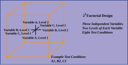
In this arrangement, called a 2×2×2 factorial design, each of the three factors would be run at two levels and all the eight possible combinations included.

The factors changed were heat treatment, outer ring osculation, and cage design.

… But, if you average the pairs of numbers for cage design, you get the [table below], which shows what the two other factors did.

"Remembering that bearings like this one have been made for decades, it is at first surprising that it could take so long to discover so important an improvement.

A likely explanation is that, because most engineers have, until recently, employed only one factor at a time experimentation, interaction effects have been missed."

As a further example, the effects of three input variables can be evaluated in eight experimental conditions shown as the corners of a cube.

For example, a shrimp aquaculture experiment[9] might have factors temperature at 25 °C and 35 °C, density at 80 or 160 shrimp/40 liters, and salinity at 10%, 25% and 40%.

In the aquaculture experiment, the ordered triple (25, 80, 10) represents the treatment combination having the lowest level of each factor.

[note 2] The expected response to a given treatment combination is called a cell mean,[12] usually denoted using the Greek letter μ.

Since the true cell means are unobservable in principle, a statistical hypothesis test is used to assess whether this expression equals 0.

Interaction in a factorial experiment is the lack of additivity between factors, and is also expressed by contrasts.

Similarly, the pattern of the B columns follows the levels of factor B (sorting on B makes this easier to see).

Similarly, the two contrast vectors for B depend only on the level of factor B, namely the second component of "cell", so they belong to the main effect of B.

For example, the entries in the B column follow the same pattern as the middle component of "cell", as can be seen by sorting on B.

Finally, the ABC column represents the three-factor interaction: its entries depend on the levels of all three factors, and it is orthogonal to the other six contrast vectors.

Replication is more common for small experiments and is a very reliable way of assessing experimental error.

However, the number of experimental runs required for three-level (or more) factorial designs will be considerably greater than for their two-level counterparts.

[21] To compute the main effect of a factor "A" in a 2-level experiment, subtract the average response of all experimental runs for which A was at its low (or first) level from the average response of all experimental runs for which A was at its high (or second) level.

When the factors are continuous, two-level factorial designs assume that the effects are linear.

If a quadratic effect is expected for a factor, a more complicated experiment should be used, such as a central composite design.

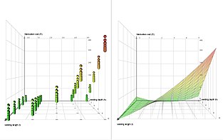
Optimization of factors that could have quadratic effects is the primary goal of response surface methodology.

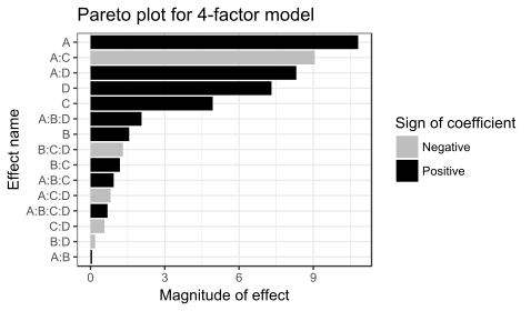
The analysis of variance (ANOVA) including all 4 factors and all possible interaction terms between them yields the coefficient estimates shown in the table below.

Because there are 16 observations and 16 coefficients (intercept, main effects, and interactions), p-values cannot be calculated for this model.