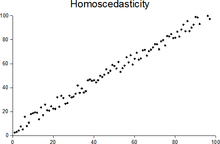
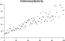
Homoscedasticity and heteroscedasticity
“Skedasticity” comes from the Ancient Greek word “skedánnymi”, meaning “to scatter”.
[1][2][3] Assuming a variable is homoscedastic when in reality it is heteroscedastic (/ˌhɛtəroʊskəˈdæstɪk/) results in unbiased but inefficient point estimates and in biased estimates of standard errors, and may result in overestimating the goodness of fit as measured by the Pearson coefficient.
The existence of heteroscedasticity is a major concern in regression analysis and the analysis of variance, as it invalidates statistical tests of significance that assume that the modelling errors all have the same variance.
While the ordinary least squares estimator is still unbiased in the presence of heteroscedasticity, it is inefficient and inference based on the assumption of homoskedasticity is misleading.
[4][5] Nowadays, standard practice in econometrics is to include Heteroskedasticity-consistent standard errors instead of using GLS, as GLS can exhibit strong bias in small samples if the actual skedastic function is unknown.
[7] The econometrician Robert Engle was awarded the 2003 Nobel Memorial Prize for Economics for his studies on regression analysis in the presence of heteroscedasticity, which led to his formulation of the autoregressive conditional heteroscedasticity (ARCH) modeling technique.
The disturbance in matrix A is homoscedastic; this is the simple case where OLS is the best linear unbiased estimator.
The disturbance in matrix D is homoscedastic because the diagonal variances are constant, even though the off-diagonal covariances are non-zero and ordinary least squares is inefficient for a different reason: serial correlation.
A classic example of heteroscedasticity is that of income versus expenditure on meals.
Therefore, people with higher incomes exhibit greater variability in expenditures on food.
After five minutes, the accuracy of the measurements may be good only to 100 m, because of the increased distance, atmospheric distortion, and a variety of other factors.
Heteroscedasticity does not cause ordinary least squares coefficient estimates to be biased, although it can cause ordinary least squares estimates of the variance (and, thus, standard errors) of the coefficients to be biased, possibly above or below the true of population variance.
Thus, regression analysis using heteroscedastic data will still provide an unbiased estimate for the relationship between the predictor variable and the outcome, but standard errors and therefore inferences obtained from data analysis are suspect.
For example, if OLS is performed on a heteroscedastic data set, yielding biased standard error estimation, a researcher might fail to reject a null hypothesis at a given significance level, when that null hypothesis was actually uncharacteristic of the actual population (making a type II error).
Heteroscedasticity is also a major practical issue encountered in ANOVA problems.
[3] One author wrote, "unequal error variance is worth correcting only when the problem is severe.
"[12] In addition, another word of caution was in the form, "heteroscedasticity has never been a reason to throw out an otherwise good model.
"[3][13] With the advent of heteroscedasticity-consistent standard errors allowing for inference without specifying the conditional second moment of error term, testing conditional homoscedasticity is not as important as in the past.
[6] For any non-linear model (for instance Logit and Probit models), however, heteroscedasticity has more severe consequences: the maximum likelihood estimates (MLE) of the parameters will usually be biased, as well as inconsistent (unless the likelihood function is modified to correctly take into account the precise form of heteroscedasticity or the distribution is a member of the linear exponential family and the conditional expectation function is correctly specified).
[14][15] Yet, in the context of binary choice models (Logit or Probit), heteroscedasticity will only result in a positive scaling effect on the asymptotic mean of the misspecified MLE (i.e. the model that ignores heteroscedasticity).
[16] As a result, the predictions which are based on the misspecified MLE will remain correct.
In addition, the misspecified Probit and Logit MLE will be asymptotically normally distributed which allows performing the usual significance tests (with the appropriate variance-covariance matrix).
However, regarding the general hypothesis testing, as pointed out by Greene, "simply computing a robust covariance matrix for an otherwise inconsistent estimator does not give it redemption.
Consequently, the virtue of a robust covariance matrix in this setting is unclear.
From this auxiliary regression, the explained sum of squares is retained, divided by two, and then becomes the test statistic for a chi-squared distribution with the degrees of freedom equal to the number of independent variables.
[22][additional citation(s) needed] From the auxiliary regression, it retains the R-squared value which is then multiplied by the sample size, and then becomes the test statistic for a chi-squared distribution (and uses the same degrees of freedom).
are both homoscedastic and lack serial correlation if they share the same diagonals in their covariance matrix,
Homoscedastic distributions are especially useful to derive statistical pattern recognition and machine learning algorithms.
One popular example of an algorithm that assumes homoscedasticity is Fisher's linear discriminant analysis.
Several authors have considered tests in this context, for both regression and grouped-data situations.