Least squares

In regression analysis, least squares is a parameter estimation method based on minimizing the sum of the squares of the residuals (a residual being the difference between an observed value and the fitted value provided by a model) made in the results of each individual equation.

The linear least-squares problem occurs in statistical regression analysis; it has a closed-form solution.

Also, by iteratively applying local quadratic approximation to the likelihood (through the Fisher information), the least-squares method may be used to fit a generalized linear model.

[5][4] The method of least squares grew out of the fields of astronomy and geodesy, as scientists and mathematicians sought to provide solutions to the challenges of navigating the Earth's oceans during the Age of Discovery.

The accurate description of the behavior of celestial bodies was the key to enabling ships to sail in open seas, where sailors could no longer rely on land sightings for navigation.

Within ten years after Legendre's publication, the method of least squares had been adopted as a standard tool in astronomy and geodesy in France, Italy, and Prussia, which constitutes an extraordinarily rapid acceptance of a scientific technique.

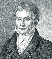
[6] In 1809 Carl Friedrich Gauss published his method of calculating the orbits of celestial bodies.

However, to Gauss's credit, he went beyond Legendre and succeeded in connecting the method of least squares with the principles of probability and to the normal distribution.

An early demonstration of the strength of Gauss's method came when it was used to predict the future location of the newly discovered asteroid Ceres.

On 1 January 1801, the Italian astronomer Giuseppe Piazzi discovered Ceres and was able to track its path for 40 days before it was lost in the glare of the Sun.

Based on these data, astronomers desired to determine the location of Ceres after it emerged from behind the Sun without solving Kepler's complicated nonlinear equations of planetary motion.

The only predictions that successfully allowed Hungarian astronomer Franz Xaver von Zach to relocate Ceres were those performed by the 24-year-old Gauss using least-squares analysis.

In 1810, after reading Gauss's work, Laplace, after proving the central limit theorem, used it to give a large sample justification for the method of least squares and the normal distribution.

In 1822, Gauss was able to state that the least-squares approach to regression analysis is optimal in the sense that in a linear model where the errors have a mean of zero, are uncorrelated, normally distributed, and have equal variances, the best linear unbiased estimator of the coefficients is the least-squares estimator.

In the next two centuries workers in the theory of errors and in statistics found many different ways of implementing least squares.

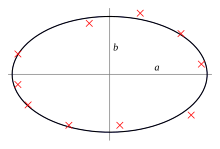
The least-squares method finds the optimal parameter values by minimizing the sum of squared residuals,

In some commonly used algorithms, at each iteration the model may be linearized by approximation to a first-order Taylor series expansion about

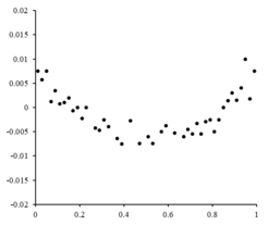
After having derived the force constant by least squares fitting, we predict the extension from Hooke's law.

In a least squares calculation with unit weights, or in linear regression, the variance on the jth parameter, denoted

where the true error variance σ2 is replaced by an estimate, the reduced chi-squared statistic, based on the minimized value of the residual sum of squares (objective function), S. The denominator, n − m, is the statistical degrees of freedom; see effective degrees of freedom for generalizations.

If the probability distribution of the parameters is known or an asymptotic approximation is made, confidence limits can be found.

In that case, a central limit theorem often nonetheless implies that the parameter estimates will be approximately normally distributed so long as the sample is reasonably large.

A special case of generalized least squares called weighted least squares occurs when all the off-diagonal entries of Ω (the correlation matrix of the residuals) are null; the variances of the observations (along the covariance matrix diagonal) may still be unequal (heteroscedasticity).

Notable statistician Sara van de Geer used empirical process theory and the Vapnik–Chervonenkis dimension to prove a least-squares estimator can be interpreted as a measure on the space of square-integrable functions.

-norm of the parameter vector, is not greater than a given value to the least squares formulation, leading to a constrained minimization problem.

This is equivalent to the unconstrained minimization problem where the objective function is the residual sum of squares plus a penalty term

[20] In a Bayesian context, this is equivalent to placing a zero-mean normally distributed prior on the parameter vector.

An alternative regularized version of least squares is Lasso (least absolute shrinkage and selection operator), which uses the constraint that

In a Bayesian context, this is equivalent to placing a zero-mean Laplace prior distribution on the parameter vector.

Some feature selection techniques are developed based on the LASSO including Bolasso which bootstraps samples,[25] and FeaLect which analyzes the regression coefficients corresponding to different values of