Maximum likelihood estimation
This is achieved by maximizing a likelihood function so that, under the assumed statistical model, the observed data is most probable.
[1] The logic of maximum likelihood is both intuitive and flexible, and as such the method has become a dominant means of statistical inference.
In some cases, the first-order conditions of the likelihood function can be solved analytically; for instance, the ordinary least squares estimator for a linear regression model maximizes the likelihood when the random errors are assumed to have normal distributions with the same variance.
[5] From the perspective of Bayesian inference, MLE is generally equivalent to maximum a posteriori (MAP) estimation with a prior distribution that is uniform in the region of interest.
In frequentist inference, MLE is a special case of an extremum estimator, with the objective function being the likelihood.
The goal of maximum likelihood estimation is to determine the parameters for which the observed data have the highest joint probability.
but in general no closed-form solution to the maximization problem is known or available, and an MLE can only be found via numerical optimization.
Conveniently, most common probability distributions – in particular the exponential family – are logarithmically concave.
[10][11] While the domain of the likelihood function—the parameter space—is generally a finite-dimensional subset of Euclidean space, additional restrictions sometimes need to be incorporated into the estimation process.
then, as a practical matter, means to find the maximum of the likelihood function subject to the constraint
Theoretically, the most natural approach to this constrained optimization problem is the method of substitution, that is "filling out" the restrictions
and we have a sufficiently large number of observations n, then it is possible to find the value of θ0 with arbitrary precision.
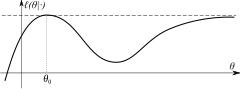
Compactness implies that the likelihood cannot approach the maximum value arbitrarily close at some other point (as demonstrated for example in the picture on the right).
is by definition[19] It maximizes the so-called profile likelihood: The MLE is also equivariant with respect to certain transformations of the data.
is the Fisher information matrix: In particular, it means that the bias of the maximum likelihood estimator is equal to zero up to the order 1/√n .
However, when we consider the higher-order terms in the expansion of the distribution of this estimator, it turns out that θmle has bias of order 1⁄n.
The Bayesian Decision theory is about designing a classifier that minimizes total expected risk, especially, when the costs (the loss function) associated with different decisions are equal, the classifier is minimizing the error over the whole distribution.
[25] Consider a case where n tickets numbered from 1 to n are placed in a box and one is selected at random (see uniform distribution); thus, the sample size is 1.
Exactly the same calculation yields s⁄n which is the maximum likelihood estimator for any sequence of n Bernoulli trials resulting in s 'successes'.
which has probability density function the corresponding probability density function for a sample of n independent identically distributed normal random variables (the likelihood) is This family of distributions has two parameters: θ = (μ, σ); so we maximize the likelihood,
Its expected value is equal to the parameter μ of the given distribution, which means that the maximum likelihood estimator
Similarly we differentiate the log-likelihood with respect to σ and equate to zero: which is solved by Inserting the estimate
we obtain To calculate its expected value, it is convenient to rewrite the expression in terms of zero-mean random variables (statistical error)
The log-likelihood of this is: The constraint has to be taken into account and use the Lagrange multipliers: By posing all the derivatives to be 0, the most natural estimate is derived Maximizing log likelihood, with and without constraints, can be an unsolvable problem in closed form, then we have to use iterative procedures.
Many methods for this kind of optimization problem are available,[26][27] but the most commonly used ones are algorithms based on an updating formula of the form where the vector
is the inverse of the Hessian matrix of the log-likelihood function, both evaluated the rth iteration.
[31][32] But because the calculation of the Hessian matrix is computationally costly, numerous alternatives have been proposed.
DFP formula finds a solution that is symmetric, positive-definite and closest to the current approximate value of second-order derivative: where BFGS also gives a solution that is symmetric and positive-definite: where BFGS method is not guaranteed to converge unless the function has a quadratic Taylor expansion near an optimum.
However, BFGS can have acceptable performance even for non-smooth optimization instances Another popular method is to replace the Hessian with the Fisher information matrix,
[34] Early users of maximum likelihood include Carl Friedrich Gauss, Pierre-Simon Laplace, Thorvald N. Thiele, and Francis Ysidro Edgeworth.