Pearson correlation coefficient
It was developed by Karl Pearson from a related idea introduced by Francis Galton in the 1880s, and for which the mathematical formula was derived and published by Auguste Bravais in 1844.
The correlation coefficient can be derived by considering the cosine of the angle between two points representing the two sets of x and y co-ordinate data.
Pearson's correlation coefficient is the covariance of the two variables divided by the product of their standard deviations.
This formula suggests a convenient single-pass algorithm for calculating sample correlations, though depending on the numbers involved, it can sometimes be numerically unstable.
[13] In case of missing data, Garren derived the maximum likelihood estimator.
A key mathematical property of the Pearson correlation coefficient is that it is invariant under separate changes in location and scale in the two variables.
More general linear transformations do change the correlation: see § Decorrelation of n random variables for an application of this.
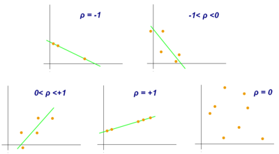
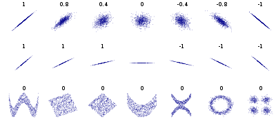
An absolute value of exactly 1 implies that a linear equation describes the relationship between X and Y perfectly, with all data points lying on a line.
The correlation coefficient is negative (anti-correlation) if Xi and Yi tend to lie on opposite sides of their respective means.
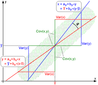
Rodgers and Nicewander[17] cataloged thirteen ways of interpreting correlation or simple functions of it: For uncentered data, there is a relation between the correlation coefficient and the angle φ between the two regression lines, y = gX(x) and x = gY(y), obtained by regressing y on x and x on y respectively.
As an example, suppose five countries are found to have gross national products of 1, 2, 3, 5, and 8 billion dollars, respectively.
A correlation of 0.8 may be very low if one is verifying a physical law using high-quality instruments, but may be regarded as very high in the social sciences, where there may be a greater contribution from complicating factors.
The p-value for the permutation test is the proportion of the r values generated in step (2) that are larger than the Pearson correlation coefficient that was calculated from the original data.
are random variables, with a simple linear relationship between them with an additive normal noise (i.e., y= a + bx + e), then a standard error associated to the correlation is where
[24] This holds approximately in case of non-normal observed values if sample sizes are large enough.
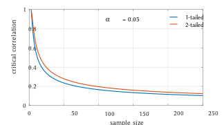
[25] For determining the critical values for r the inverse function is needed: Alternatively, large sample, asymptotic approaches can be used.
Another early paper[26] provides graphs and tables for general values of ρ, for small sample sizes, and discusses computational approaches.
In the case where the underlying variables are not normal, the sampling distribution of Pearson's correlation coefficient follows a Student's t-distribution, but the degrees of freedom are reduced.
For example, if z = 2.2 is observed and a two-sided p-value is desired to test the null hypothesis that
For example, suppose we observe r = 0.7 with a sample size of n=50, and we wish to obtain a 95% confidence interval for ρ.
then as a starting point the total variation in the Yi around their average value can be decomposed as follows where the
This can be rearranged to give The two summands above are the fraction of variance in Y that is explained by X (right) and that is unexplained by X (left).
Thus, the sample correlation coefficient between the observed and fitted response values in the regression can be written (calculation is under expectation, assumes Gaussian statistics) Thus where
In some practical applications, such as those involving data suspected to follow a heavy-tailed distribution, this is an important consideration.
However, the existence of the correlation coefficient is usually not a concern; for instance, if the range of the distribution is bounded, ρ is always defined.
Note however that while most robust estimators of association measure statistical dependence in some way, they are generally not interpretable on the same scale as the Pearson correlation coefficient.
These non-parametric approaches may give more meaningful results in some situations where bivariate normality does not hold.
A stratified analysis is one way to either accommodate a lack of bivariate normality, or to isolate the correlation resulting from one factor while controlling for another.
If W represents cluster membership or another factor that it is desirable to control, we can stratify the data based on the value of W, then calculate a correlation coefficient within each stratum.
The Pearson distance has been used in cluster analysis and data detection for communications and storage with unknown gain and offset.