Robust statistics
Robust statistical methods have been developed for many common problems, such as estimating location, scale, and regression parameters.
In statistics, classical estimation methods rely heavily on assumptions that are often not met in practice.
Unfortunately, when there are outliers in the data, classical estimators often have very poor performance, when judged using the breakdown point and the influence function described below.
The practical effect of problems seen in the influence function can be studied empirically by examining the sampling distribution of proposed estimators under a mixture model, where one mixes in a small amount (1–5% is often sufficient) of contamination.
Strictly speaking, a robust statistic is resistant to errors in the results, produced by deviations from assumptions[4] (e.g., of normality).
By contrast, more robust estimators that are not so sensitive to distributional distortions such as longtailedness are also resistant to the presence of outliers.
Thus, if the mean is intended as a measure of the location of the center of the data, it is, in a sense, biased when outliers are present.
This simple example demonstrates that when outliers are present, the standard deviation cannot be recommended as an estimate of scale.
Care must be taken; initial data showing the ozone hole first appearing over Antarctica were rejected as outliers by non-human screening.
The basic tools used to describe and measure robustness are the breakdown point, the influence function and the sensitivity curve.
The X% trimmed mean has a breakdown point of X%, for the chosen level of X. Huber (1981) and Maronna et al. (2019) contain more details.
We can divide this by the square root of the sample size to get a robust standard error, and we find this quantity to be 0.78.
Thus, the change in the mean resulting from removing two outliers is approximately twice the robust standard error.
The empirical influence function is a measure of the dependence of the estimator on the value of any one of the points in the sample.
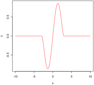
Properties of an influence function that bestow it with desirable performance are: This value, which looks a lot like a Lipschitz constant, represents the effect of shifting an observation slightly from
It can be shown that M-estimators are asymptotically normally distributed so that as long as their standard errors can be computed, an approximate approach to inference is available.
Since M-estimators are normal only asymptotically, for small sample sizes it might be appropriate to use an alternative approach to inference, such as the bootstrap.
Of course, as we saw with the speed-of-light example, the mean is only normally distributed asymptotically and when outliers are present the approximation can be very poor even for quite large samples.
For the speed-of-light data, allowing the kurtosis parameter to vary and maximizing the likelihood, we get Fixing
and maximizing the likelihood gives A pivotal quantity is a function of data, whose underlying population distribution is a member of a parametric family, that is not dependent on the values of the parameters.
[13] In addition, outliers can sometimes be accommodated in the data through the use of trimmed means, other scale estimators apart from standard deviation (e.g., MAD) and Winsorization.
The accuracy of the estimate depends on how good and representative the model is and how long the period of missing values extends.
The Kohonen self organising map (KSOM) offers a simple and robust multivariate model for data analysis, thus providing good possibilities to estimate missing values, taking into account their relationship or correlation with other pertinent variables in the data record.
To this end Ting, Theodorou & Schaal (2007) have recently shown that a modification of Masreliez's theorem can deal with outliers.
[18] Although influence functions have a long history in statistics, they were not widely used in machine learning due to several challenges.
One of the primary obstacles is that traditional influence functions rely on expensive second-order derivative computations and assume model differentiability and convexity.
These assumptions are limiting, especially in modern machine learning, where models are often non-differentiable, non-convex, and operate in high-dimensional spaces.
Koh & Liang (2017) addressed these challenges by introducing methods to efficiently approximate influence functions using second-order optimization techniques, such as those developed by Pearlmutter (1994), Martens (2010), and Agarwal, Bullins & Hazan (2017).
Their approach remains effective even when the assumptions of differentiability and convexity degrade, enabling influence functions to be used in the context of non-convex deep learning models.
They demonstrated that influence functions are a powerful and versatile tool that can be applied to a variety of tasks in machine learning, including: Koh and Liang’s contributions have opened the door for influence functions to be used in various applications across machine learning, from interpretability to security, marking a significant advance in their applicability.