Spearman's rank correlation coefficient

ranks are distinct integers (no ties), it can be computed using the popular formula where Consider a bivariate sample

Observe now that Putting this all together thus yields Identical values are usually[7] each assigned fractional ranks equal to the average of their positions in the ascending order of the values, which is equivalent to averaging over all possible permutations.

If ties are present in the data set, the simplified formula above yields incorrect results: Only if in both variables all ranks are distinct, then

The simplified method should also not be used in cases where the data set is truncated; that is, when the Spearman's correlation coefficient is desired for the top X records (whether by pre-change rank or post-change rank, or both), the user should use the Pearson correlation coefficient formula given above.

[8] There are several other numerical measures that quantify the extent of statistical dependence between pairs of observations.

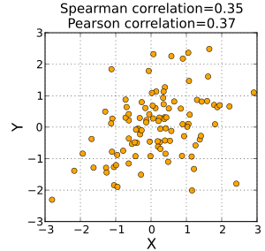
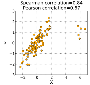
The Spearman correlation increases in magnitude as X and Y become closer to being perfectly monotonic functions of each other.

A perfectly monotonic increasing relationship implies that for any two pairs of data values Xi, Yi and Xj, Yj, that Xi − Xj and Yi − Yj always have the same sign.

A perfectly monotonic decreasing relationship implies that these differences always have opposite signs.

First, a perfect Spearman correlation results when X and Y are related by any monotonic function.

Contrast this with the Pearson correlation, which only gives a perfect value when X and Y are related by a linear function.

In this example, the arbitrary raw data in the table below is used to calculate the correlation between the IQ of a person with the number of hours spent in front of TV per week [fictitious values used].

These values can now be substituted back into the equation to give which evaluates to ρ = −29/165 = −0.175757575... with a p-value = 0.627188 (using the t-distribution).

That the value is close to zero shows that the correlation between IQ and hours spent watching TV is very low, although the negative value suggests that the longer the time spent watching television the lower the IQ.

Confidence intervals for Spearman's ρ can be easily obtained using the Jackknife Euclidean likelihood approach in de Carvalho and Marques (2012).

One approach to test whether an observed value of ρ is significantly different from zero (r will always maintain −1 ≤ r ≤ 1) is to calculate the probability that it would be greater than or equal to the observed r, given the null hypothesis, by using a permutation test.

An advantage of this approach is that it automatically takes into account the number of tied data values in the sample and the way they are treated in computing the rank correlation.

Another approach parallels the use of the Fisher transformation in the case of the Pearson product-moment correlation coefficient.

That is, confidence intervals and hypothesis tests relating to the population value ρ can be carried out using the Fisher transformation: If F(r) is the Fisher transformation of r, the sample Spearman rank correlation coefficient, and n is the sample size, then is a z-score for r, which approximately follows a standard normal distribution under the null hypothesis of statistical independence (ρ = 0).

[12][13] One can also test for significance using which is distributed approximately as Student's t-distribution with n − 2 degrees of freedom under the null hypothesis.

Classic correspondence analysis is a statistical method that gives a score to every value of two nominal variables.

There exists an equivalent of this method, called grade correspondence analysis, which maximizes Spearman's ρ or Kendall's τ.

[17] There are two existing approaches to approximating the Spearman's rank correlation coefficient from streaming data.

stores the number of observations that fall into the two-dimensional cell indexed by

For non-stationary streaming data, where the Spearman's rank correlation coefficient may change over time, the same procedure can be applied, but to a moving window of observations.

The second approach to approximating the Spearman's rank correlation coefficient from streaming data involves the use of Hermite series based estimators.

This estimator is phrased in terms of linear algebra operations for computational efficiency (equation (8) and algorithm 1 and 2[19]).

These algorithms are only applicable to continuous random variable data, but have certain advantages over the count matrix approach in this setting.

The first advantage is improved accuracy when applied to large numbers of observations.

The second advantage is that the Spearman's rank correlation coefficient can be computed on non-stationary streams without relying on a moving window.

Instead, the Hermite series based estimator uses an exponential weighting scheme to track time-varying Spearman's rank correlation from streaming data, which has constant memory requirements with respect to "effective" moving window size.