Spectral density estimation
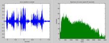
[1] Intuitively speaking, the spectral density characterizes the frequency content of the signal.
Some SDE techniques assume that a signal is composed of a limited (usually small) number of generating frequencies plus noise and seek to find the location and intensity of the generated frequencies.
Others make no assumption on the number of components and seek to estimate the whole generating spectrum.
Any process that quantifies the various amounts (e.g. amplitudes, powers, intensities) versus frequency (or phase) can be called spectrum analysis.
General mathematical techniques for analyzing non-periodic functions fall into the category of Fourier analysis.
The Fourier transform of a function produces a frequency spectrum which contains all of the information about the original signal, but in a different form.
This means that the original function can be completely reconstructed (synthesized) by an inverse Fourier transform.
For perfect reconstruction, the spectrum analyzer must preserve both the amplitude and phase of each frequency component.
These two pieces of information can be represented as a 2-dimensional vector, as a complex number, or as magnitude (amplitude) and phase in polar coordinates (i.e., as a phasor).
Frequency analysis also simplifies the understanding and interpretation of the effects of various time-domain operations, both linear and non-linear.
In practice, nearly all software and electronic devices that generate frequency spectra utilize a discrete Fourier transform (DFT), which operates on samples of the signal, and which provides a mathematical approximation to the full integral solution.
The DFT is almost invariably implemented by an efficient algorithm called fast Fourier transform (FFT).
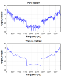
The array of squared-magnitude components of a DFT is a type of power spectrum called periodogram, which is widely used for examining the frequency characteristics of noise-free functions such as filter impulse responses and window functions.
But the periodogram does not provide processing-gain when applied to noiselike signals or even sinusoids at low signal-to-noise ratios[why?].
In other words, the variance of its spectral estimate at a given frequency does not decrease as the number of samples used in the computation increases.
This can be mitigated by averaging over time (Welch's method[2]) or over frequency (smoothing).
Welch's method is widely used for spectral density estimation (SDE).
However, periodogram-based techniques introduce small biases that are unacceptable in some applications.
Many other techniques for spectral estimation have been developed to mitigate the disadvantages of the basic periodogram.
These techniques can generally be divided into non-parametric, parametric, and more recently semi-parametric (also called sparse) methods.
By contrast, the parametric approaches assume that the underlying stationary stochastic process has a certain structure that can be described using a small number of parameters (for example, using an auto-regressive or moving-average model).
In these approaches, the task is to estimate the parameters of the model that describes the stochastic process.
Similar approaches may also be used for missing data recovery[4] as well as signal reconstruction.
If one only wants to estimate the frequency of the single loudest pure-tone signal, one can use a pitch detection algorithm.
Methods for instantaneous frequency estimation include those based on the Wigner–Ville distribution and higher order ambiguity functions.
The most common methods for frequency estimation involve identifying the noise subspace to extract these components.
Suppose that it is a sum of a finite number of periodic components (all frequencies are positive): The variance of
is, for a zero-mean function as above, given by If these data were samples taken from an electrical signal, this would be its average power (power is energy per unit time, so it is analogous to variance if energy is analogous to the amplitude squared).
Now, for simplicity, suppose the signal extends infinitely in time, so we pass to the limit as
If the average power is bounded, which is almost always the case in reality, then the following limit exists and is the variance of the data.