Survival analysis

Survival analysis is a branch of statistics for analyzing the expected duration of time until one event occurs, such as death in biological organisms and failure in mechanical systems.

Even in biological problems, some events (for example, heart attack or other organ failure) may have the same ambiguity.

The study of recurring events is relevant in systems reliability, and in many areas of social sciences and medical research.

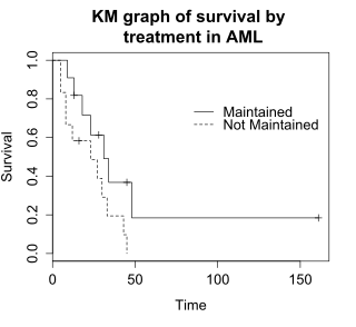
The graph shows the KM plot for the aml data and can be interpreted as follows: A life table summarizes survival data in terms of the number of events and the proportion surviving at each event time point.

The columns in the life table have the following interpretation: The log-rank test compares the survival times of two or more groups.

This example uses a log-rank test for a difference in survival in the maintained versus non-maintained treatment groups in the aml data.

The sample size of 23 subjects is modest, so there is little power to detect differences between the treatment groups.

The chi-squared test is based on asymptotic approximation, so the p-value should be regarded with caution for small sample sizes.

The log-rank test and KM curves don't work easily with quantitative predictors such as gene expression, white blood count, or age.

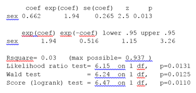
For quantitative predictor variables, an alternative method is Cox proportional hazards regression analysis.

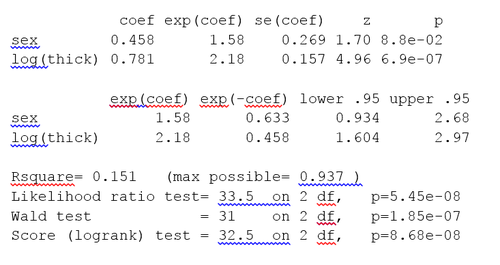
The Cox proportional hazards regression using R gives the results shown in the box.

The Likelihood ratio test has better behavior for small sample sizes, so it is generally preferred.

The Cox model extends the log-rank test by allowing the inclusion of additional covariates.

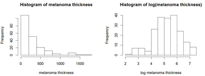
In the histograms, the thickness values are positively skewed and do not have a Gaussian-like, Symmetric probability distribution.

Specifically, these methods assume that a single line, curve, plane, or surface is sufficient to separate groups (alive, dead) or to estimate a quantitative response (survival time).

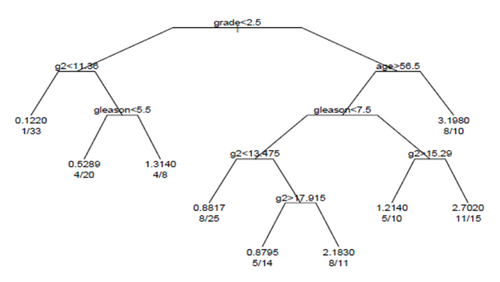
[8] The example is based on 146 stage C prostate cancer patients in the data set stagec in rpart.

[10] The randomForestSRC package includes an example survival random forest analysis using the data set pbc.

This data is from the Mayo Clinic Primary Biliary Cirrhosis (PBC) trial of the liver conducted between 1974 and 1984.

Deep learning approaches have shown superior performance especially on complex input data modalities such as images and clinical time-series.

The object of primary interest is the survival function, conventionally denoted S, which is defined as

The survival function is usually assumed to approach zero as age increases without bound (i.e., S(t) → 0 as t → ∞), although the limit could be greater than zero if eternal life is possible.

The age at which a specified proportion of survivors remain can be found by solving the equation S(t) = q for t, where q is the quantile in question.

Right censoring will occur, for example, for those subjects whose birth date is known but who are still alive when they are lost to follow-up or when the study ends.

If the event of interest has already happened before the subject is included in the study but it is not known when it occurred, the data is said to be left-censored.

Indeed, time to HIV seroconversion can be determined only by a laboratory assessment which is usually initiated after a visit to the physician.

The same is true for the diagnosis of AIDS, which is based on clinical symptoms and needs to be confirmed by a medical examination.

Although we may know the right-hand side of the duration of interest, we may never know the exact time of exposure to the infectious agent.

However, computing the likelihood function (needed for fitting parameters or making other kinds of inferences) is complicated by the censoring.

The likelihood function for a survival model, in the presence of censored data, is formulated as follows.

Periodic case (cohort) and death (and recovery) counts are statistically sufficient to make nonparametric maximum likelihood and least squares estimates of survival functions, without lifetime data.