t-distributed stochastic neighbor embedding
t-distributed stochastic neighbor embedding (t-SNE) is a statistical method for visualizing high-dimensional data by giving each datapoint a location in a two or three-dimensional map.
It is based on Stochastic Neighbor Embedding originally developed by Geoffrey Hinton and Sam Roweis,[1] where Laurens van der Maaten and Hinton proposed the t-distributed variant.
[2] It is a nonlinear dimensionality reduction technique for embedding high-dimensional data for visualization in a low-dimensional space of two or three dimensions.
Specifically, it models each high-dimensional object by a two- or three-dimensional point in such a way that similar objects are modeled by nearby points and dissimilar objects are modeled by distant points with high probability.
The t-SNE algorithm comprises two main stages.
First, t-SNE constructs a probability distribution over pairs of high-dimensional objects in such a way that similar objects are assigned a higher probability while dissimilar points are assigned a lower probability.
Second, t-SNE defines a similar probability distribution over the points in the low-dimensional map, and it minimizes the Kullback–Leibler divergence (KL divergence) between the two distributions with respect to the locations of the points in the map.
While the original algorithm uses the Euclidean distance between objects as the base of its similarity metric, this can be changed as appropriate.
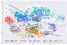
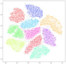
t-SNE has been used for visualization in a wide range of applications, including genomics, computer security research,[3] natural language processing, music analysis,[4] cancer research,[5] bioinformatics,[6] geological domain interpretation,[7][8][9] and biomedical signal processing.
[10] For a data set with n elements, t-SNE runs in O(n2) time and requires O(n2) space.
As van der Maaten and Hinton explained: "The similarity of datapoint
from the N samples are estimated as 1/N, so the conditional probability can be written as
is set in such a way that the entropy of the conditional distribution equals a predefined entropy using the bisection method.
As a result, the bandwidth is adapted to the density of the data: smaller values of
are used in denser parts of the data space.
The entropy increases with the perplexity of this distribution
The perplexity is a hand-chosen parameter of t-SNE, and as the authors state, "perplexity can be interpreted as a smooth measure of the effective number of neighbors.
The performance of SNE is fairly robust to changes in the perplexity, and typical values are between 5 and 50.".
[2] Since the Gaussian kernel uses the Euclidean distance
, it is affected by the curse of dimensionality, and in high dimensional data when distances lose the ability to discriminate, the
become too similar (asymptotically, they would converge to a constant).
It has been proposed to adjust the distances with a power transform, based on the intrinsic dimension of each point, to alleviate this.
typically chosen as 2 or 3) that reflects the similarities
Herein a heavy-tailed Student t-distribution (with one-degree of freedom, which is the same as a Cauchy distribution) is used to measure similarities between low-dimensional points in order to allow dissimilar objects to be modeled far apart in the map.
in the map are determined by minimizing the (non-symmetric) Kullback–Leibler divergence of the distribution
, that is: The minimization of the Kullback–Leibler divergence with respect to the points
The result of this optimization is a map that reflects the similarities between the high-dimensional inputs.
While t-SNE plots often seem to display clusters, the visual clusters can be strongly influenced by the chosen parameterization (especially the perplexity) and so a good understanding of the parameters for t-SNE is needed.
[14] Thus, interactive exploration may be needed to choose parameters and validate results.
[15][16] It has been shown that t-SNE can often recover well-separated clusters, and with special parameter choices, approximates a simple form of spectral clustering.