Time constant
In physics and engineering, the time constant, usually denoted by the Greek letter τ (tau), is the parameter characterizing the response to a step input of a first-order, linear time-invariant (LTI) system.
[1][note 1] The time constant is the main characteristic unit of a first-order LTI system.
[2] In the frequency domain (for example, looking at the Fourier transform of the step response, or using an input that is a simple sinusoidal function of time) the time constant also determines the bandwidth of a first-order time-invariant system, that is, the frequency at which the output signal power drops to half the value it has at low frequencies.
The time constant is also used to characterize the frequency response of various signal processing systems – magnetic tapes, radio transmitters and receivers, record cutting and replay equipment, and digital filters – which can be modelled or approximated by first-order LTI systems.
Time constants are a feature of the lumped system analysis (lumped capacity analysis method) for thermal systems, used when objects cool or warm uniformly under the influence of convective cooling or warming.
where τ represents the exponential decay constant and V is a function of time t
An example solution to the differential equation with initial value V0 and no forcing function is
is the initial value of V. Thus, the response is an exponential decay with time constant τ.
Here: After a period of one time constant the function reaches e−1 = approximately 37% of its initial value.
In case 4, after five time constants the function reaches a value less than 1% of its original.
In most cases this 1% threshold is considered sufficient to assume that the function has decayed to zero – as a rule of thumb, in control engineering a stable system is one that exhibits such an overall damped behavior.
By convention, the bandwidth of this system is the frequency where |V∞|2 drops to half-value, or where ωτ = 1.
This is the usual bandwidth convention, defined as the frequency range where power drops by less than half (at most −3 dB).
Simply stated, a system approaches its final, steady-state situation at a constant rate, regardless of how close it is to that value at any arbitrary starting point.
For example, consider an electric motor whose startup is well modelled by a first-order LTI system.
In an RL circuit composed of a single resistor and inductor, the time constant
Similarly, in an RC circuit composed of a single resistor and capacitor, the time constant
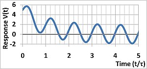
In the case where feedback is present, a system may exhibit unstable, increasing oscillations.
[4] Time constants are a feature of the lumped system analysis (lumped capacity analysis method) for thermal systems, used when objects cool or warm uniformly under the influence of convective cooling or warming.
The negative sign indicates the temperature drops when the heat transfer is outward from the body (that is, when F > 0).
In other words, larger masses ρV with higher heat capacities cp lead to slower changes in temperature (longer time constant τ), while larger surface areas As with higher heat transfer h lead to more rapid temperature change (shorter time constant τ).
Comparison with the introductory differential equation suggests the possible generalization to time-varying ambient temperatures Ta.
However, retaining the simple constant ambient example, by substituting the variable ΔT ≡ (T − Ta), one finds:
In words, the body assumes the same temperature as the ambient at an exponentially slow rate determined by the time constant.
In an excitable cell such as a muscle or neuron, the time constant of the membrane potential
Vmax is defined as the maximum voltage change from the resting potential, where
The larger a time constant is, the slower the rise or fall of the potential of a neuron.
A short time constant rather produces a coincidence detector through spatial summation.
In exponential decay, such as of a radioactive isotope, the time constant can be interpreted as the mean lifetime.
A time constant is the amount of time it takes for a meteorological sensor to respond to a rapid change in a measure, and until it is measuring values within the accuracy tolerance usually expected of the sensor.