Numerical weather prediction

Manipulating the vast datasets and performing the complex calculations necessary to modern numerical weather prediction requires some of the most powerful supercomputers in the world.

Post-processing techniques such as model output statistics (MOS) have been developed to improve the handling of errors in numerical predictions.

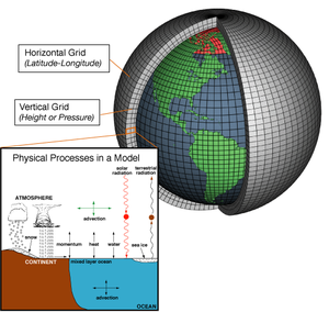
In addition, the partial differential equations used in the model need to be supplemented with parameterizations for solar radiation, moist processes (clouds and precipitation), heat exchange, soil, vegetation, surface water, and the effects of terrain.

The history of numerical weather prediction began in the 1920s through the efforts of Lewis Fry Richardson, who used procedures originally developed by Vilhelm Bjerknes[1] to produce by hand a six-hour forecast for the state of the atmosphere over two points in central Europe, taking at least six weeks to do so.

The ENIAC was used to create the first weather forecasts via computer in 1950, based on a highly simplified approximation to the atmospheric governing equations.

[4][5] In 1954, Carl-Gustav Rossby's group at the Swedish Meteorological and Hydrological Institute used the same model to produce the first operational forecast (i.e., a routine prediction for practical use).

[10] The first general circulation climate model that combined both oceanic and atmospheric processes was developed in the late 1960s at the NOAA Geophysical Fluid Dynamics Laboratory.

[1][12] The development of limited area (regional) models facilitated advances in forecasting the tracks of tropical cyclones as well as air quality in the 1970s and 1980s.

[15] The output of forecast models based on atmospheric dynamics is unable to resolve some details of the weather near the Earth's surface.

On land, terrain maps available at resolutions down to 1 kilometer (0.6 mi) globally are used to help model atmospheric circulations within regions of rugged topography, in order to better depict features such as downslope winds, mountain waves and related cloudiness that affects incoming solar radiation.

[21] One main source of input is observations from devices (called radiosondes) in weather balloons which rise through the troposphere and well into the stratosphere that measure various atmospheric parameters and transmits them to a fixed receiver.

[24] These observations are irregularly spaced, so they are processed by data assimilation and objective analysis methods, which perform quality control and obtain values at locations usable by the model's mathematical algorithms.

[29][30] Reconnaissance aircraft are also flown over the open oceans during the cold season into systems which cause significant uncertainty in forecast guidance, or are expected to be of high impact from three to seven days into the future over the downstream continent.

[32] Efforts to involve sea surface temperature in model initialization began in 1972 due to its role in modulating weather in higher latitudes of the Pacific.

A typical cumulus cloud has a scale of less than 1 kilometer (0.6 mi), and would require a grid even finer than this to be represented physically by the equations of fluid motion.

[46] The amount of solar radiation reaching the ground, as well as the formation of cloud droplets occur on the molecular scale, and so they must be parameterized before they can be included in the model.

[50] Within air quality models, parameterizations take into account atmospheric emissions from multiple relatively tiny sources (e.g. roads, fields, factories) within specific grid boxes.

[61] Extremely small errors in temperature, winds, or other initial inputs given to numerical models will amplify and double every five days,[61] making it impossible for long-range forecasts—those made more than two weeks in advance—to predict the state of the atmosphere with any degree of forecast skill.

Furthermore, existing observation networks have poor coverage in some regions (for example, over large bodies of water such as the Pacific Ocean), which introduces uncertainty into the true initial state of the atmosphere.

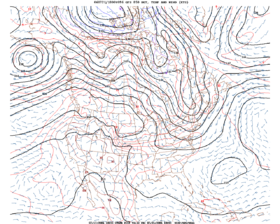
Ensemble spread is diagnosed through tools such as spaghetti diagrams, which show the dispersion of one quantity on prognostic charts for specific time steps in the future.

[72] Air quality forecasting attempts to predict when the concentrations of pollutants will attain levels that are hazardous to public health.

[73] In addition to pollutant source and terrain information, these models require data about the state of the fluid flow in the atmosphere to determine its transport and diffusion.

[76] Versions designed for climate applications with time scales of decades to centuries were originally created in 1969 by Syukuro Manabe and Kirk Bryan at the Geophysical Fluid Dynamics Laboratory in Princeton, New Jersey.

[77] When run for multiple decades, computational limitations mean that the models must use a coarse grid that leaves smaller-scale interactions unresolved.

[84] Because weather drifts across the world, producing forecasts a week or more in advance typically involves running a numerical prediction model for the entire planet.

On a molecular scale, there are two main competing reaction processes involved in the degradation of cellulose, or wood fuels, in wildfires.

When there is a low amount of moisture in a cellulose fiber, volatilization of the fuel occurs; this process will generate intermediate gaseous products that will ultimately be the source of combustion.

The chemical kinetics of both reactions indicate that there is a point at which the level of moisture is low enough—and/or heating rates high enough—for combustion processes to become self-sufficient.

Consequently, changes in wind speed, direction, moisture, temperature, or lapse rate at different levels of the atmosphere can have a significant impact on the behavior and growth of a wildfire.

Numerical weather models have limited forecast skill at spatial resolutions under 1 kilometer (0.6 mi), forcing complex wildfire models to parameterize the fire in order to calculate how the winds will be modified locally by the wildfire, and to use those modified winds to determine the rate at which the fire will spread locally.