Logistic regression
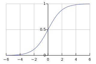
More abstractly, the logistic function is the natural parameter for the Bernoulli distribution, and in this sense is the "simplest" way to convert a real number to a probability.
For example, the Trauma and Injury Severity Score (TRISS), which is widely used to predict mortality in injured patients, was originally developed by Boyd et al. using logistic regression.
Logistic regression is a supervised machine learning algorithm widely used for binary classification tasks, such as identifying whether an email is spam or not and diagnosing diseases by assessing the presence or absence of specific conditions based on patient test results.
This approach utilizes the logistic (or sigmoid) function to transform a linear combination of input features into a probability value ranging between 0 and 1.
By calculating the probability that the dependent variable will be categorized into a specific group, logistic regression provides a probabilistic framework that supports informed decision-making.
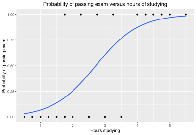
[20] As a simple example, we can use a logistic regression with one explanatory variable and two categories to answer the following question: A group of 20 students spends between 0 and 6 hours studying for an exam.
The reason for using logistic regression for this problem is that the values of the dependent variable, pass and fail, while represented by "1" and "0", are not cardinal numbers.
We wish to fit a logistic function to the data consisting of the hours studied (xk) and the outcome of the test (yk =1 for pass, 0 for fail).
of the predictors) as follows: For a continuous independent variable the odds ratio can be defined as: This exponential relationship provides an interpretation for
For the simple binary logistic regression model, we assumed a linear relationship between the predictor variable and the log-odds (also called logit) of the event that
[25] The interpretation of the βj parameter estimates is as the additive effect on the log of the odds for a unit change in the j the explanatory variable.
It turns out that this formulation is exactly equivalent to the preceding one, phrased in terms of the generalized linear model and without any latent variables.
The reason for this separation is that it makes it easy to extend logistic regression to multi-outcome categorical variables, as in the multinomial logit model.
On the other hand, the left-of-center party might be expected to raise taxes and offset it with increased welfare and other assistance for the lower and middle classes.
[26][27] Unlike linear regression with normally distributed residuals, it is not possible to find a closed-form expression for the coefficient values that maximize the likelihood function so an iterative process must be used instead; for example Newton's method.
A failure to converge may occur for a number of reasons: having a large ratio of predictors to cases, multicollinearity, sparseness, or complete separation.
) can, for example, be calculated using iteratively reweighted least squares (IRLS), which is equivalent to maximizing the log-likelihood of a Bernoulli distributed process using Newton's method.
Now, though, automatic software such as OpenBUGS, JAGS, PyMC, Stan or Turing.jl allows these posteriors to be computed using simulation, so lack of conjugacy is not a concern.
[33] Also, one can argue that 96 observations are needed only to estimate the model's intercept precisely enough that the margin of error in predicted probabilities is ±0.1 with a 0.95 confidence level.
For example, in simple linear regression, a set of K data points (xk, yk) are fitted to a proposed model function of the form
In the case of simple binary logistic regression, the set of K data points are fitted in a probabilistic sense to a function of the form: where
[35] In linear regression the squared multiple correlation, R2 is used to assess goodness of fit as it represents the proportion of variance in the criterion that is explained by the predictors.
This test is considered to be obsolete by some statisticians because of its dependence on arbitrary binning of predicted probabilities and relative low power.
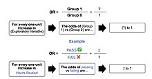
Given that the logit is not intuitive, researchers are likely to focus on a predictor's effect on the exponential function of the regression coefficient – the odds ratio (see definition).
An important point is that the probabilities are treated equally and the fact that they sum to 1 is part of the Lagrangian formulation, rather than being assumed from the beginning.
Rather than being specific to the assumed multinomial logistic case, it is taken to be a general statement of the condition at which the log-likelihood is maximized and makes no reference to the functional form of pnk.
[46][47] In his more detailed paper (1845), Verhulst determined the three parameters of the model by making the curve pass through three observed points, which yielded poor predictions.
They were initially unaware of Verhulst's work and presumably learned about it from L. Gustave du Pasquier, but they gave him little credit and did not adopt his terminology.
[52] Pearl and Reed first applied the model to the population of the United States, and also initially fitted the curve by making it pass through three points; as with Verhulst, this again yielded poor results.
[58] In 1973 Daniel McFadden linked the multinomial logit to the theory of discrete choice, specifically Luce's choice axiom, showing that the multinomial logit followed from the assumption of independence of irrelevant alternatives and interpreting odds of alternatives as relative preferences;[59] this gave a theoretical foundation for the logistic regression.