Standard deviation

In statistics, the standard deviation is a measure of the amount of variation of the values of a variable about its mean.

The standard deviation of a random variable, sample, statistical population, data set, or probability distribution is the square root of its variance.

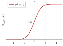
If the population of interest is approximately normally distributed, the standard deviation provides information on the proportion of observations above or below certain values.

If the distribution has fat tails going out to infinity, the standard deviation might not exist, because the integral might not converge.

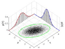
The standard deviation of a continuous real-valued random variable X with probability density function p(x) is

In the case of a parametric family of distributions, the standard deviation can be expressed in terms of the parameters.

This estimator also has a uniformly smaller mean squared error than the corrected sample standard deviation.

This estimator is unbiased if the variance exists and the sample values are drawn independently with replacement.

For unbiased estimation of standard deviation, there is no formula that works across all distributions, unlike for mean and variance.

For the normal distribution, an unbiased estimator is given by ⁠s/c4⁠, where the correction factor (which depends on N) is given in terms of the Gamma function, and equals:

To show how a larger sample will make the confidence interval narrower, consider the following examples: A small population of N = 2 has only one degree of freedom for estimating the standard deviation.

is the p-th quantile of the chi-square distribution with k degrees of freedom, and 1 − α is the confidence level.

These same formulae can be used to obtain confidence intervals on the variance of residuals from a least squares fit under standard normal theory, where k is now the number of degrees of freedom for error.

For a set of N > 4 data spanning a range of values R, an upper bound on the standard deviation s is given by s = 0.6R.

See computational formula for the variance for proof, and for an analogous result for the sample standard deviation.

This makes sense since they fall outside the range of values that could reasonably be expected to occur if the prediction were correct and the standard deviation appropriately quantified.

By using standard deviations, a minimum and maximum value can be calculated that the averaged weight will be within some very high percentage of the time (99.9% or more).

A five-sigma level translates to one chance in 3.5 million that a random fluctuation would yield the result.

This level of certainty was required in order to assert that a particle consistent with the Higgs boson had been discovered in two independent experiments at CERN,[11] also leading to the declaration of the first observation of gravitational waves.

[12] As a simple example, consider the average daily maximum temperatures for two cities, one inland and one on the coast.

In finance, standard deviation is often used as a measure of the risk associated with price-fluctuations of a given asset (stocks, bonds, property, etc.

Stock A over the past 20 years had an average return of 10 percent, with a standard deviation of 20 percentage points (pp) and Stock B, over the same period, had average returns of 12 percent but a higher standard deviation of 30 pp.

Squaring the difference in each period and taking the average gives the overall variance of the return of the asset.

Finding the square root of this variance will give the standard deviation of the investment tool in question.

The standard deviation therefore is simply a scaling variable that adjusts how broad the curve will be, though it also appears in the normalizing constant.

For example, if a series of 10 measurements of a previously unknown quantity is performed in a laboratory, it is possible to calculate the resulting sample mean and sample standard deviation, but it is impossible to calculate the standard deviation of the mean.

Applying this method to a time series will result in successive values of standard deviation corresponding to n data points as n grows larger with each new sample, rather than a constant-width sliding window calculation.

s0 is now the sum of the weights and not the number of samples N. The incremental method with reduced rounding errors can also be applied, with some additional complexity.

[19][20] This was as a replacement for earlier alternative names for the same idea: for example, Gauss used mean error.

[21] The standard deviation index (SDI) is used in external quality assessments, particularly for medical laboratories.