Q–Q plot
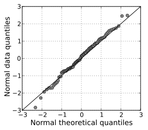
If the two distributions being compared are similar, the points in the Q–Q plot will approximately lie on the identity line y = x.
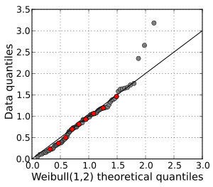
If the distributions are linearly related, the points in the Q–Q plot will approximately lie on a line, but not necessarily on the line y = x. Q–Q plots can also be used as a graphical means of estimating parameters in a location-scale family of distributions.
A Q–Q plot is generally more diagnostic than comparing the samples' histograms, but is less widely known.
Q–Q plots are commonly used to compare a data set to a theoretical model.
[2][3] This can provide an assessment of goodness of fit that is graphical, rather than reducing to a numerical summary statistic.
A more complicated construction is the case where two data sets of different sizes are being compared.
For distributions with a single shape parameter, the probability plot correlation coefficient plot provides a method for estimating the shape parameter – one simply computes the correlation coefficient for different values of the shape parameter, and uses the one with the best fit, just as if one were comparing distributions of different types.
[6] Many other choices have been suggested, both formal and heuristic, based on theory or simulations relevant in context.
More generally, Shapiro–Wilk test uses the expected values of the order statistics of the given distribution; the resulting plot and line yields the generalized least squares estimate for location and scale (from the intercept and slope of the fitted line).
However, this requires calculating the expected values of the order statistic, which may be difficult if the distribution is not normal.
Alternatively, one may use estimates of the median of the order statistics, which one can compute based on estimates of the median of the order statistics of a uniform distribution and the quantile function of the distribution; this was suggested by Filliben (1975).
[9] This can be easily generated for any distribution for which the quantile function can be computed, but conversely the resulting estimates of location and scale are no longer precisely the least squares estimates, though these only differ significantly for n small.
These can be expressed in terms of the quantile function and the order statistic medians for the continuous uniform distribution by: where U(i) are the uniform order statistic medians and G is the quantile function for the desired distribution.
The R programming language comes with functions to make Q–Q plots, namely qqnorm and qqplot from the stats package.
The fastqq package implements faster plotting for large number of data points.